Table of Content
5. Resampling Methods
Resampling methods are an indispensable tool in modern statistics. They involve repeatedly drawing samples from a training set and refitting a model of interest on each sample in order to obtain additional information about the fitted model. For example, in order to estimate the variability of a linear regression fit, we can repeatedly draw different samples from the training data, fit a linear regression to each new sample, and then examine the extent to which the resulting fits differ. Such an approach may allow us to obtain information that would not be available from fitting the model only once using the original training sample.
Resampling approaches can be computationally expensive, because they involve fitting the same statistical method multiple times using different subsets of the training data. However, due to recent advances in computing power, the computational requirements of resampling methods generally are not prohibitive. In this chapter, we discuss two of the most commonly used resampling methods, cross-validation and the bootstrap. Both methods are important tools in the practical application of many statistical learning procedures.
For example, cross-validation can be used to estimate the test error associated with a given statistical learning method in order to evaluate its performance, or to select the appropriate level of flexibility. The process of evaluating a model’s performance is known as model assessment, whereas the process of selecting the proper level of flexibility for a model is known as model selection. The bootstrap is used in several contexts, most commonly to provide a measure of accuracy of a parameter estimate or of a given statistical learning method.
-----------------------------------------------------------
5.1 Cross-Validation
-----------------------------------------------------------
In Chapter 2 we discuss the distinction between the test error rate and the training error rate. The test error is the average error that results from using a statistical learning method to predict the response on a new observation that is, a measurement that was not used in training the method. Given a data set, the use of a particular statistical learning method is warranted if it results in a low test error. The test error can be easily calculated if a designated test set is available. Unfortunately, this is usually not the case. In contrast, the training error can be easily calculated by applying the statistical learning method to the observations used in its training. But as we saw in Chapter 2, the training error rate often is quite different from the test error rate, and in particular the former can dramatically underestimate the latter.
Directly estimate the test error rate, a number of techniques can be used to estimate this quantity using the available training data. Some methods make a mathematical adjustment to the training error rate in order to estimate the test error rate. Such approaches are discussed in Chapter 6. In this section, we instead consider a class of methods that estimate the test error rate by holding out a subset of the training observations from the fitting process, and then applying the statistical learning method to those held out observations.
-----------------------------------------------------------
5.1.1 The Validation Set Approach
-----------------------------------------------------------
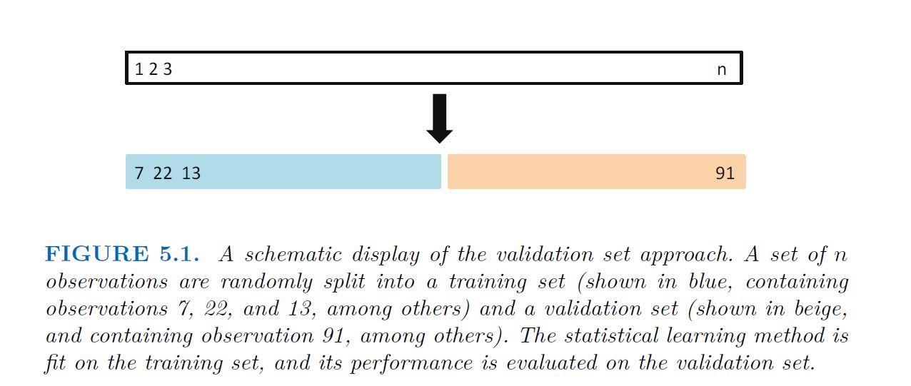
fitting a particular statistical learning method on a set of observations. The validation set approach, displayed in Figure 5.1, is a very simple strategy for this task. It involves randomly dividing the available set of observations into two parts, a training set and a validation set or hold-out set.
The model is fit on the training set, and the fitted model is used to predict the responses for the observations in the validation set. The resulting validation set error rate typically assessed using MSE in the case of a quantitative response provides an estimate of the test error rate.
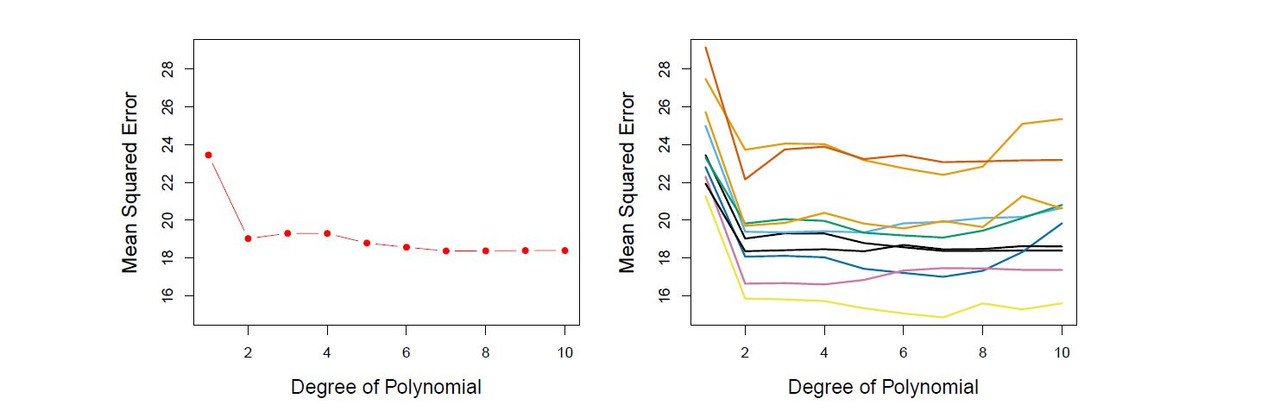
Recall that in order to create the left-hand panel of Figure 5.2, we randomly divided the data set into two parts, a training set and a validation set. If we repeat the process of randomly splitting the sample set into two parts, we will get a somewhat different estimate for the test MSE. As an illustration, the right-hand panel of Figure 5.2 displays ten different validation set MSE curves from the Auto data set, produced using ten different random splits of the observations into training and validation sets. All ten curves indicate that the model with a quadratic term has a dramatically smaller validation set MSE than the model with only a linear term. Furthermore, all ten curves indicate that there is not much benefit in including cubic or higher-order polynomial terms in the model. But it is worth noting that each of the ten curves results in a different test MSE estimate for each of the ten regression models considered. And there is no consensus among the curves as to which model results in the smallest validation set MSE. Based on the variability among these curves, all that we can conclude with any confidence is that the linear fit is not adequate for this data.
The validation set approach is conceptually simple and is easy to implement. But it has two potential drawbacks:
As is shown in the right-hand panel of Figure 5.2, the validation estimate of the test error rate can be highly variable, depending on precisely which observations are included in the training set and which observations are included in the validation set. In the validation approach, only a subset of the observations—those that are included in the training set rather than in the validation set—are used to fit the model. Since statistical methods tend to perform worse when trained on fewer observations, this suggests that the validation set error rate may tend to overestimate the test error rate for the model fit on the entire data set.
-----------------------------------------------------------
5.1.2 Leave-One-Out Cross-Validation
-----------------------------------------------------------
Leave-one-out cross-validation (LOOCV) is closely related to the validation set approach of Section 5.1.1, but it attempts to address that method’s drawbacks.
Like the validation set approach, LOOCV involves splitting the set of observations into two parts. However, instead of creating two subsets of comparable size, a single observation (x1, y1) is used for the validation set, and the remaining observations {(x2, y2), . . . , (xn, yn)} make up the training set. The statistical learning method is fit on the n − 1 training observations, and a prediction $\hat{y}_1$ is made for the excluded observation, using its value x1. Since (x1, y1) was not used in the fitting process, MSE1 = $(y_1 - \hat{y}_1)^2$ provides an approximately unbiased estimate for the test error. But even though MSE1 is unbiased for the test error, it is a poor estimate because it is highly variable, since it is based upon a single observation (x1, y1).
We can repeat the procedure by selecting (x2, y2) for the validation data, training the statistical learning procedure on the n − 1 observations {(x1, y1), (x3, y3), . . . , (xn, yn)}, and computing MSE2 = (y2 - y^2)² . Repeating this approach n times produces n squared errors, MSE1, . . . , MSEn. The LOOCV estimate for the test MSE is the average of these n test error estimates:

A schematic of the LOOCV approach is illustrated in Figure 5.3. LOOCV has a couple of major advantages over the validation set approach. First, it has far less bias. In LOOCV, we repeatedly fit the statistical learning method using training sets that contain n − 1 observations, almost as many as are in the entire data set. This is in contrast to the validation set approach, in which the training set is typically around half the size of the original data set. Consequently, the LOOCV approach tends not to overestimate the test error rate as much as the validation set approach does. Second, in contrast to the validation approach which will yield different results when applied repeatedly due to randomness in the training/validation set splits, performing LOOCV multiple times will always yield the same results: there is no randomness in the training/validation set splits.
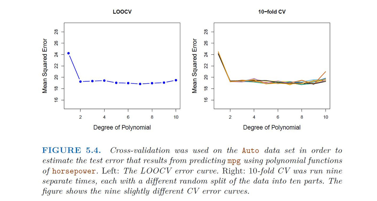
We used LOOCV on the Auto data set in order to obtain an estimate of the test set MSE that results from fitting a linear regression model to predict mpg using polynomial functions of horsepower.
LOOCV has the potential to be expensive to implement, since the model has to be fit n times. This can be very time consuming if n is large, and if each individual model is slow to fit. With least squares linear or polynomial regression, an amazing shortcut makes the cost of LOOCV the same as that of a single model fit! The following formula holds:


-----------------------------------------------------------
5.1.3 k-Fold Cross-Validation
-----------------------------------------------------------
An alternative to LOOCV is k-fold CV. This approach involves randomly dividing the set of observations into k groups, or folds, of approximately equal size. The first fold is treated as a validation set, and the method is fit on the remaining k − 1 folds. The mean squared error, MSE1, is then computed on the observations in the held-out fold. This procedure is repeated k times; each time, a different group of observations is treated as a validation set. This process results in k estimates of the test error, MSE1,MSE2, . . . ,MSEk. The k-fold CV estimate is computed by averaging these values,.


It is not hard to see that LOOCV is a special case of k-fold CV in which k is set to equal n. In practice, one typically performs k-fold CV using k = 5 or k = 10. What is the advantage of using k = 5 or k = 10 rather than k = n? The most obvious advantage is computational. LOOCV requires fitting the statistical learning method n times. This has the potential to be computationally expensive (except for linear models fit by least squares, in which case formula (5.2) can be used). But cross-validation is a very general approach that can be applied to almost any statistical learning method. Some statistical learning methods have computationally intensive fitting procedures, and so performing LOOCV may pose computational problems, especially if n is extremely large. In contrast, performing 10-fold CV requires fitting the learning procedure only ten times, which may be much more feasible. As we see in Section 5.1.4, there also can be other non-computational advantages to performing 5-fold or 10-fold CV, which involve the bias-variance trade-off.
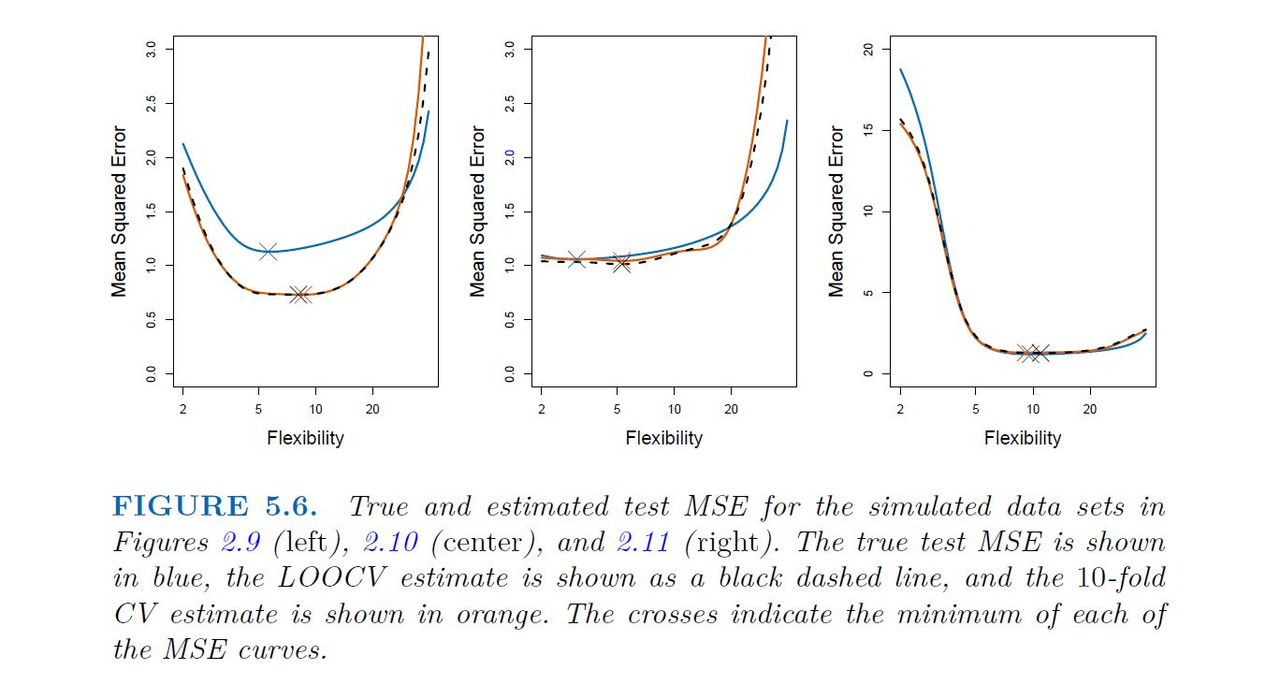
When we perform cross-validation, our goal might be to determine how well a given statistical learning procedure can be expected to perform on independent data; in this case, the actual estimate of the test MSE is of interest. But at other times we are interested only in the location of the minimum point in the estimated test MSE curve. This is because we might be performing cross-validation on a number of statistical learning methods, or on a single method using different levels of flexibility, in order to identify the method that results in the lowest test error. For this purpose, the location of the minimum point in the estimated test MSE curve is important, but the actual value of the estimated test MSE is not. We find in Figure 5.6 that despite the fact that they sometimes underestimate the true test MSE, all of the CV curves come close to identifying the correct level of flexibility that is, the flexibility level corresponding to the smallest test MSE.
-----------------------------------------------------------
5.1.4 Bias-Variance Trade-Off for k-Fold Cross-Validation
-----------------------------------------------------------
We mentioned in Section 5.1.3 that k-fold CV with k < n has a computational advantage to LOOCV. But putting computational issues aside, a less obvious but potentially more important advantage of k-fold CV is that it often gives more accurate estimates of the test error rate than does LOOCV. This has to do with a bias-variance trade-off.
It was mentioned in Section 5.1.1 that the validation set approach can lead to overestimates of the test error rate, since in this approach the training set used to fit the statistical learning method contains only half the observations of the entire data set. Using this logic, it is not hard to see that LOOCV will give approximately unbiased estimates of the test error, since each training set contains n−1 observations, which is almost as many as the number of observations in the full data set. And performing k-fold CV for, say, k = 5 or k = 10 will lead to an intermediate level of bias, since each training set contains approximately (k − 1)n/k observations fewer than in the LOOCV approach, but substantially more than in the validation set approach. Therefore, from the perspective of bias reduction, it is clear that LOOCV is to be preferred to k-fold CV.
However, we know that bias is not the only source for concern in an estimating procedure; we must also consider the procedure’s variance. It turns out that LOOCV has higher variance than does k-fold CV with k < n. Why is this the case? When we perform LOOCV, we are in effect averaging the outputs of n fitted models, each of which is trained on an almost identical set of observations; therefore, these outputs are highly (positively) correlated with each other. In contrast, when we perform k-fold CV with k < n, we are averaging the outputs of k fitted models that are somewhat less correlated with each other, since the overlap between the training sets in each model is smaller. Since the mean of many highly correlated quantities has higher variance than does the mean of many quantities that are not as highly correlated, the test error estimate resulting from LOOCV tends to have higher variance than does the test error estimate resulting from k-fold CV.
To summarize, there is a bias-variance trade-off associated with the choice of k in k-fold cross-validation. Typically, given these considerations, one performs k-fold cross-validation using k = 5 or k = 10, as these values have been shown empirically to yield test error rate estimates that suffer neither from excessively high bias nor from very high variance.
-----------------------------------------------------------
5.1.5 Cross-Validation on Classification Problems
-----------------------------------------------------------
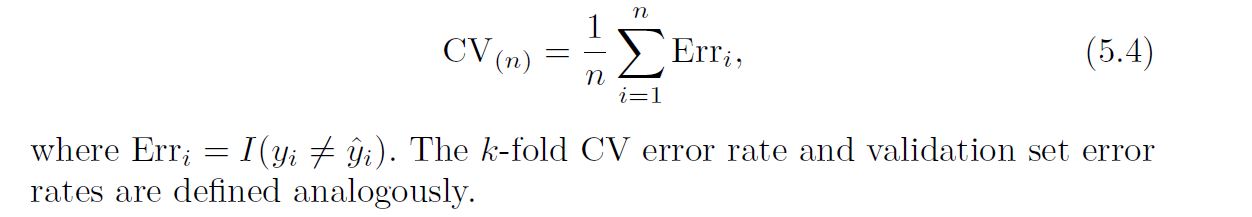
In this chapter so far, we have illustrated the use of cross-validation in the regression setting where the outcome Y is quantitative, and so have used MSE to quantify test error. But cross-validation can also be a very useful approach in the classification setting when Y is qualitative. In this setting, cross-validation works just as described earlier in this chapter, except that rather than using MSE to quantify test error, we instead use the number of misclassified observations. For instance, in the classification setting, the LOOCV error rate takes the form:
As an example, we fit various logistic regression models on the two dimensional classification data displayed in Figure 2.13. In the top-left panel of Figure 5.7, the black solid line shows the estimated decision boundary resulting from fitting a standard logistic regression model to this data set. Since this is simulated data, we can compute the true test error rate, which takes a value of 0.201 and so is substantially larger than the Bayes error rate of 0.133.
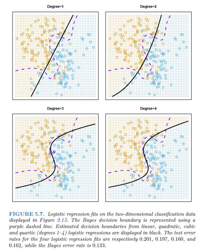
Clearly logistic regression does not have enough flexibility to model the Bayes decision boundary in this setting. We can easily extend logistic regression to obtain a non-linear decision boundary by using polynomial functions of the predictors, as we did in the regression setting in Section 3.3.2. For example, we can fit a quadratic logistic regression model, given by:

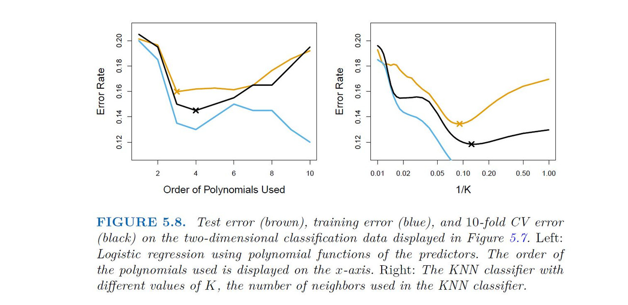
In practice, for real data, the Bayes decision boundary and the test error rates are unknown. So how might we decide between the four logistic regression models displayed in Figure 5.7? We can use cross-validation in order to make this decision. The left-hand panel of Figure 5.8 displays in black the 10-fold CV error rates that result from fitting ten logistic regression models to the data, using polynomial functions of the predictors up to tenth order. The true test errors are shown in brown, and the training errors are shown in blue. As we have seen previously, the training error tends to decrease as the flexibility of the fit increases. (The figure indicates that though the training error rate doesn’t quite decrease monotonically, it tends to decrease on the whole as the model complexity increases.) In contrast, the test error displays a characteristic U-shape. The 10-fold CV error rate provides a pretty good approximation to the test error rate. While it somewhat underestimates the error rate, it reaches a minimum when fourth-order polynomials are used, which is very close to the minimum of the test curve, which occurs when third-order polynomials are used. In fact, using fourth-order polynomials would likely lead to good test set performance, as the true test error rate is approximately the same for third, fourth, fifth, and sixth-order polynomials.
The right-hand panel of Figure 5.8 displays the same three curves using the KNN approach for classification, as a function of the value of K (which in this context indicates the number of neighbors used in the KNN classifier, rather than the number of CV folds used). Again the training error rate declines as the method becomes more flexible, and so we see that the training error rate cannot be used to select the optimal value for K. Though the cross-validation error curve slightly underestimates the test error rate, it takes on a minimum very close to the best value for K.
Correct vs. Wrong Use of Cross-Validation (CV)
Examples of Correct and Wrong Use of Cross-Validation with Predictor Filtering
Correct Use of Cross-Validation with Predictor Filtering
Scenario:
You are working on a classification problem with 50 predictors (features). You want to use cross-validation and filter out irrelevant predictors to improve the model's performance.
Correct Approach:
Apply Cross-Validation First:
- Use K-Fold or other CV techniques to split your data into training and testing sets.
Within Each Fold:
Perform Predictor Filtering (Feature Selection): Select important predictors only on the training set (e.g., using methods like correlation-based filtering, recursive feature elimination, or regularization).
Train the Model: Fit the model using the selected predictors from the training set.
Evaluate on the Test Set: Use the test set from the current fold (which hasn’t seen any filtering) to evaluate model performance.
Repeat for All Folds: After CV completes, calculate the overall performance based on all the test sets.
Why This is Correct:
The model is trained and tested in a way that reflects real-world scenarios (test data is not used for filtering).
No data leakage occurs because predictor filtering happens within the cross-validation loop on the training set only.
Wrong Use of Cross-Validation with Predictor Filtering
Scenario:
You want to reduce the number of predictors from 50 to a smaller set using feature selection, but you apply the filtering before cross-validation.
Wrong Approach:
Perform Predictor Filtering on the Entire Dataset First:
- You select important features (e.g., by calculating correlations or using a feature selection algorithm) on the entire dataset, including the test data.
Apply Cross-Validation After Filtering:
- Now, you split the data into training and testing sets for cross-validation, but the feature selection was already done on the full dataset.
Why This is Wrong:
Data Leakage: The feature selection process had access to the entire dataset, including the test set, during filtering. This allows the model to "cheat" by learning from data that should have been unseen during training.
Overestimated Performance: Since the predictors were selected with information from the test set, the cross-validation results will be overly optimistic and won’t reflect the real-world performance of the model on new, unseen data.
Summary
| Correct Use | Wrong Use |
| 1. Split data into folds using cross-validation. | 1. Perform feature selection before splitting the data. |
| 2. In each fold, perform predictor filtering on the training set. | 2. Apply cross-validation after predictors were already selected. |
| 3. Train the model using the selected predictors from the training set. | 3. Feature selection is biased because it used the entire dataset. |
| 4. Evaluate the model on the test set for that fold (unseen by filtering). | 4. The test set is indirectly used during training, leading to overestimation of model performance. |
Key Point: Always perform predictor filtering within the cross-validation loop to ensure your model doesn’t "see" the test data before it’s supposed to.
-----------------------------------------------------------
5.2 The Bootstrap
-----------------------------------------------------------
The bootstrap is a widely applicable and extremely powerful statistical tool that can be used to quantify the uncertainty associated with a given estimator or statistical learning method. As a simple example, the bootstrap can be used to estimate the standard errors of the coefficients from a linear regression fit. In the specific case of linear regression, this is not particularly useful, since we saw in Chapter 3 that standard statistical software such as R outputs such standard errors automatically. However, the power of the bootstrap lies in the fact that it can be easily applied to a wide range of statistical learning methods, including some for which a measure of variability is otherwise difficult to obtain and is not automatically output by statistical software.
Suppose that we wish to invest a fixed sum of money in two financial assets that yield returns of X and Y , respectively, where X and Y are random quantities. We will invest a fraction ) of our money in X, and will invest the remaining 1 − α in Y . Since there is variability associated with the returns on these two assets, we wish to choose ) to minimize the total risk, or variance, of our investment. In other words, we want to minimize Var()X +(1−α)Y ). One can show that the value that minimizes the risk is given by
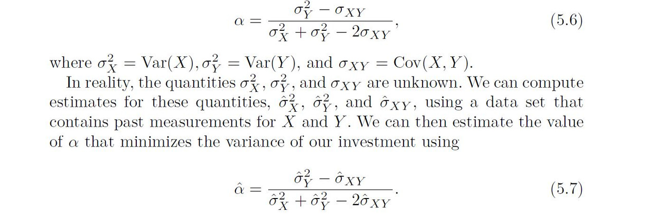
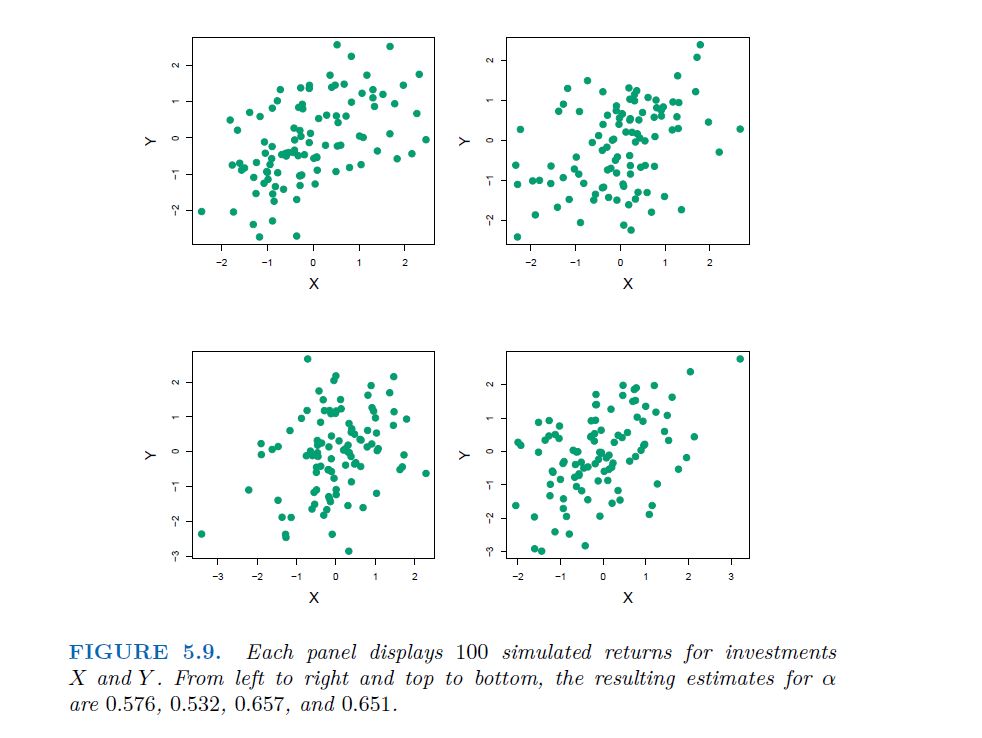
Figure 5.9 illustrates this approach for estimating $\alpha$ on a simulated data set. In each panel, we simulated 100 pairs of returns for the investments X and Y . We used these returns to estimate α²x , α²y and αxy , which we then substituted into (5.7) in order to obtain estimates for α The value of α^ resulting from each simulated data set ranges from 0.532 t
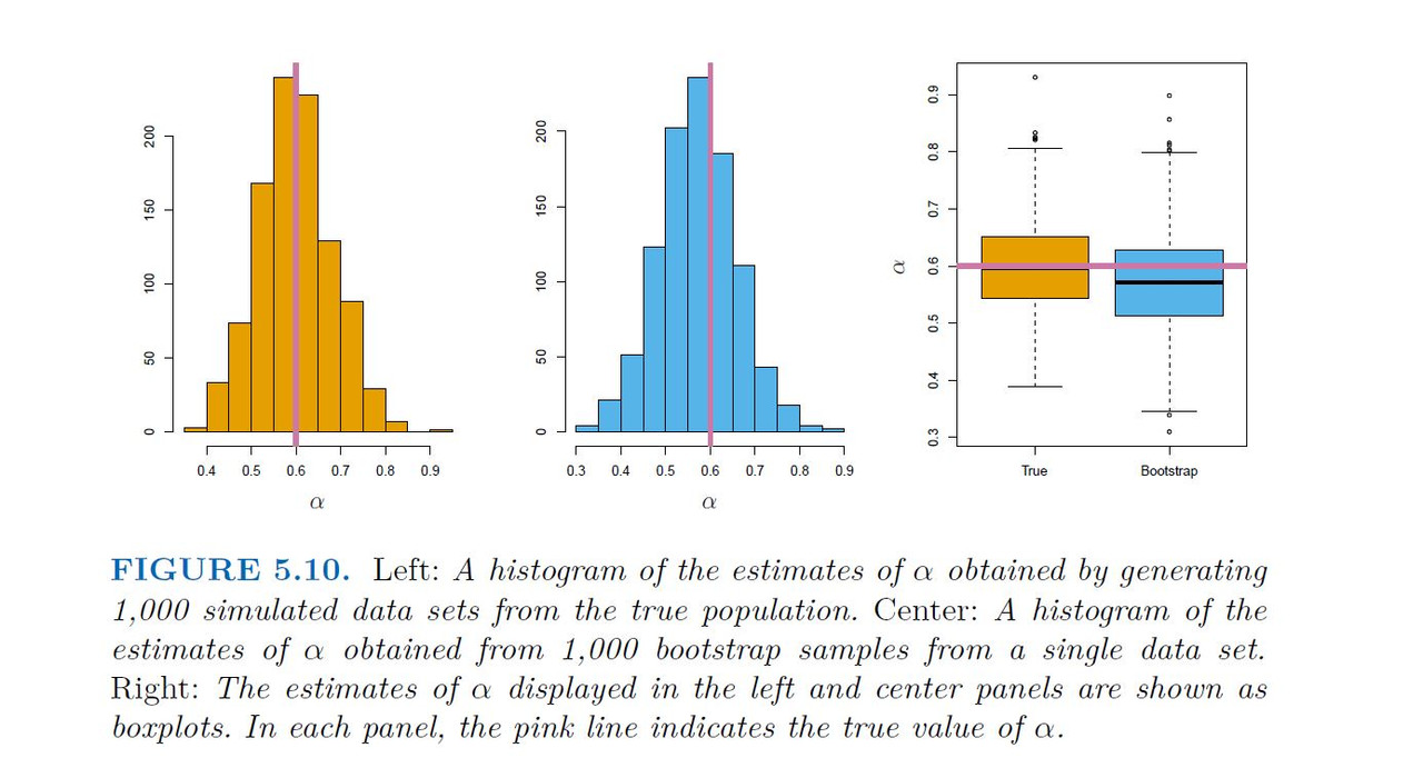
It is natural to wish to quantify the accuracy of our estimate of $\alpha$. To estimate the standard deviation of α^ , we repeated the process of simulating 100 paired observations of X and Y , and estimating α using (5.7), 1,000 times. We thereby obtained 1,000 estimates for α, which we can call α^1 ,α², . . . , α^1000. The left-hand panel of Figure 5.10 displays a histogram of the resulting estimates. For these simulations the parameters were set to α²x = 1,α²y= 1.25 and αxy = 0.5 and so we know that the true value of α is 0.6. We indicated this value using a solid vertical line on the histogram.
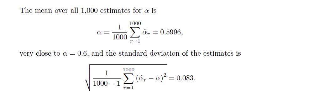
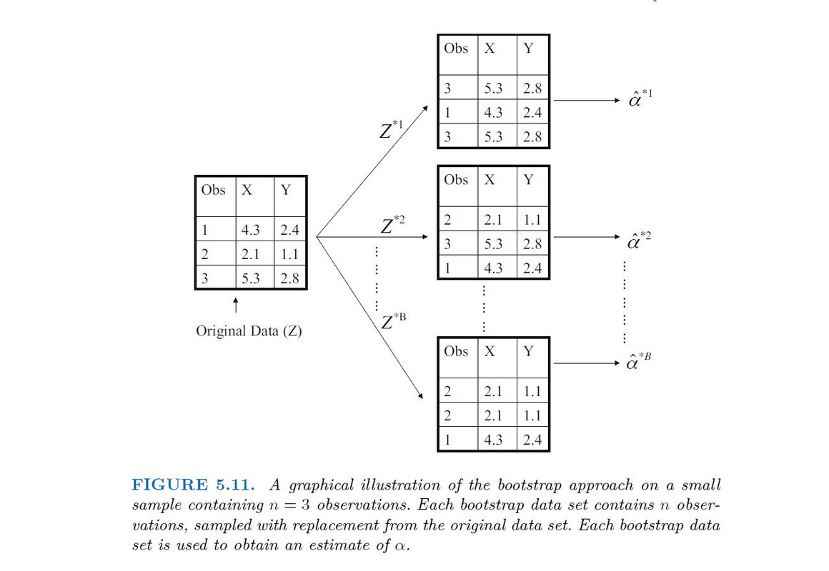
This gives us a very good idea of the accuracy of α^: SE(α^) ≈ 0.083. So roughly speaking, for a random sample from the population, we would expect α^ to differ from α by approximately 0.08, on average. In practice, however, the procedure for estimating SE(α^) outlined above cannot be applied, because for real data we cannot generate new samples from the original population. However, the bootstrap approach allows us to use a computer to emulate the process of obtaining new sample sets, so that we can estimate the variability of α^ without generating additional samples. Rather than repeatedly obtaining independent data sets from the population, we instead obtain distinct data sets by repeatedly sampling observations from the original data set
This approach is illustrated in Figure 5.11 on a simple data set, which we call Z, that contains only n = 3 observations. We randomly select n observations from the data set in order to produce a bootstrap data set, Z*1. The sampling is performed with replacement, which means that the same observation can occur more than once in the bootstrap data set.