Table of Content
4. Classification
------------------------------------------------------------------------
4.1 An Overview of Classification.
------------------------------------------------------------------------
Classification problems occur often, perhaps even more so than regression problems for Example:
A person arrives at the emergency room with a set of symptoms that could possibly be attributed to one of three medical conditions. Which of the three conditions does the individual have?
An online banking service must be able to determine whether or not a transaction being performed on the site is fraudulent, on the based of the user’s IP address, past transaction history, and so forth.
On the basis of DNA sequence data for a number of patients with and without a given disease, a biologist would like to figure out which DNA mutations are deleterious (disease-causing) and which are n
------------------------------------------------------------------------
4.2 Why Not Linear Regression?
------------------------------------------------------------------------
We have stated that linear regression is not appropriate in the case of a qualitative response. Why not? Suppose that we are trying to predict the medical condition of a patient in the emergency room on the basis of her symptoms. In this simplified example, there are three possible diagnoses: stroke, drug overdose, and epileptic seizure. We could consider encoding these values as aquantitative response variable,Y as follows:
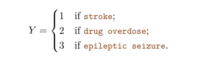
Using this coding, least squares could be used to ft a linear regression model to predict Y on the basis of a set of predictors X1,...,Xp. Unfortunately, this coding implies an ordering on the outcomes, putting drug overdose in between stroke and epileptic seizure, and insisting that the difference between stroke and drug overdose is the same as the difference between drug overdose and epileptic seizure. In practice there is no particular reason that this needs to be the case. For instance, one could choose an equally reasonable coding
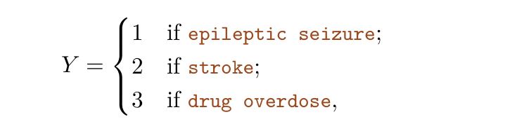
which would imply a totally different relationship among the three conditions. Each of these coding would produce fundamentally different linear models that would ultimately lead to different sets of predictions on test observations.
If the response variable’s values did take on a natural ordering, such as mild, moderate, and severe, and we felt the gap between mild and moderate was similar to the gap between moderate and severe, then a 1, 2, 3 coding would be reasonable. Unfortunately, in general there is no natural way convert a qualitative response variable with more than two levels into a quantitative response that is ready for linear regression to
------------------------------------------------------------------------
4.3 Logistic Regression
------------------------------------------------------------------------
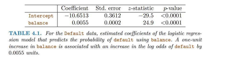
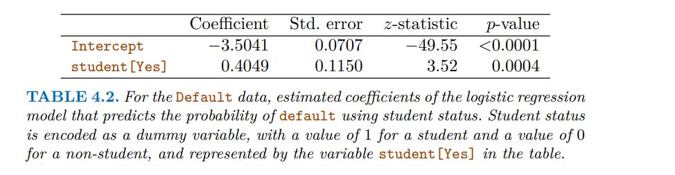
Consider again the Default data set, where the response default falls into one of two categories, Yes or No. Rather than modeling this response Y directly, logistic regression models the probability that Y belongs to a particular category.
For the Default data, logistic regression models the probability of default. For example, the probability of default given balance can be written as
Pr(default = Yes|balance).
For example, one might predict default = Yes
for any individual for whom p(balance) > 0.5. Alternatively, if a company wishes to be conservative in predicting individuals who are at risk for default, then they may choose to use a lower threshold, such as p(balance) > 0.1.
------------------------------------------------------------------------
4.3.1 The Logistic Model
------------------------------------------------------------------------
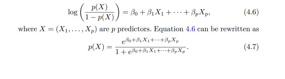
In logistic regression, we use the logistic function,


------------------------------------------------------------------------
4.3.2 Estimating the Regression Coefficients
------------------------------------------------------------------------
------------------------------------------------------------------------
4.3.4 Multiple Logistic Regression
------------------------------------------------------------------------
We now consider the problem of predicting a binary response using multiple predictors. By analogy with the extension from simple to multiple linear regression in Chapter 3, we can generalize (4.4) as follows:
Multiple Logistic Regression model results interpretation
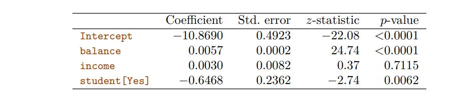
1. Balance:
For each one-unit increase in the balance, the log-odds of the dependent variable being 1 increases by 0.0057. Since the p-value is less than 0.0001, this variable is statistically significant, indicating that balance has a significant impact on the outcome
2. Income:
For each one-unit increase in income, the log-odds of the dependent variable being 1 increases by 0.0030. However, the high p-value (0.7115) suggests that income is not statistically significant in predicting the outcome, meaning its effect could be due to chance.
3. Student [Yes]:
Being a student (Yes) decreases the log-odds of the dependent variable being 1 by 0.6468. The p-value (0.0062) indicates that this variable is statistically significant, meaning student status has a significant effect on the outcome.
Summary
(The balance and student status variables are significant predictors of the outcome.)
(Income does not appear to be a significant predictor in this model.)
(The signs of the coefficients indicate the direction of the relationship with the dependent variable: positive for balance and negative for student status.)
------------------------------------------------------------------------
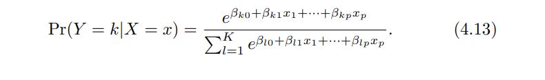
4.3.5 Multinomial Logistic Regression
------------------------------------------------------------------------
We sometimes wish to classify a response variable that has more than two classes. For example, we had three categories of medical condition in the emergency room: stroke, drug overdose, epileptic seizure.
However, the logistic regression approach that we have seen in this section only allows for K = 2 classes for the response variable.
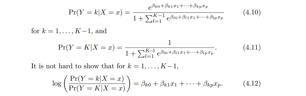
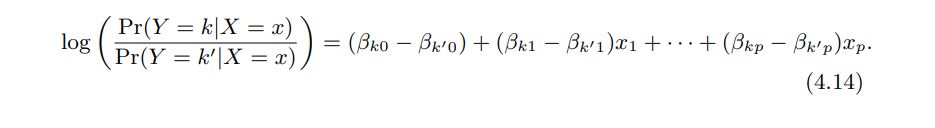
It turns out that it is possible to extend the two-class logistic regression approach to the setting of K > 2 classes. This extension is sometimes known as multinomial logistic regression. To do this, we first select a single class to serve as the baseline; without loss of generality, we select the Kth class for this role. Then we replace the model with the following model
------------------------------------------------------------------------
4.4 Generative Models for Classification
------------------------------------------------------------------------
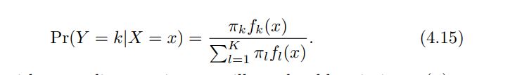
Logistic regression involves directly modeling Pr(Y = k|X = x) using the logistic function, . In statistical jargon, we model the conditional distribution of the response Y , given the predictor(s) X. We now consider an alternative and less direct approach to estimating these probabilities.
In this new approach, we model the distribution of the predictors X separately in each of the response classes (i.e. for each value of Y ). We then use Bayes’ theorem to fip these around into estimates for Pr(Y = k|X = x). When the distribution of X within each class is assumed to be normal, it turns out that the model is very similar in form to logistic regression
Why do we need another method, when we have logistic regression?
There are several reasons:
1. When there is substantial separation between the two classes, the
parameter estimates for the logistic regression model are surprisingly unstable. The methods that we consider in this section do not suffer from this problem.
2. If the distribution of the predictors X is approximately normal in
each of the classes and the sample size is small, then the approaches in this section may be more accurate than logistic regression.
3. The methods in this section can be naturally extended to the case
of more than two response classes. (In the case of more than two response classes, we can also use multinomial logistic regression from Section 4.3.5.)
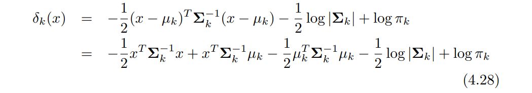
Suppose that we wish to classify an observation into one of K classes, where K ≥ 2. In other words, the qualitative response variable Y can take on K possible distinct and unordered values. Let πk represent the overall or prior probability that a randomly chosen observation comes from the kth class. Let fk(X) ≡ Pr(X|Y = k)1 denote the density function of X for an observation that comes from the kth class. In other words, fk(x) is relatively large if there is a high probability that an observation in the kth class has X ≈ x, and fk(x) is small if it is very unlikely that an observation in the kth class has X ≈ x. Then Bayes’ theorem states that In accordance with our earlier notation, we will use the abbreviation pk(x) = Pr(Y = k|X = x); this is the posterior probability that an observation X = x belongs to the kth class. That is, it is the probability that the observation belongs to the kth class, given the predictor value for that observation
------------------------------------------------------------------------
4.4.1 Linear Discriminant Analysis for p = 1
------------------------------------------------------------------------
The Gaussian density has the form
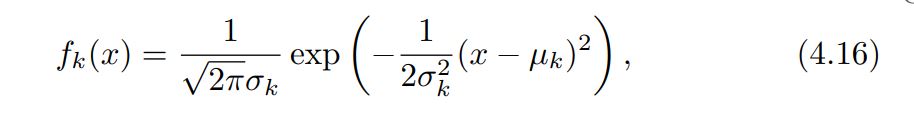
Here $\mu_{k}$ is the mean and $\sigma_{k}^2$ the variance (in class k). We will assume that all the $\sigma^2$ = $\sigma$ are the same
Plugging this into Bayes formula, we get a rather complex expression of pk(x) = Pr(y=k | X=x)

------------------------------------------------------------------------
4.4.2 Linear Discriminant Analysis for p >1
------------------------------------------------------------------------
We now extend the LDA classifier to the case of multiple predictors. To do this, we will assume that X = (X1, X2,...,Xp) is drawn from a multivariate Gaussian (or multivariate normal) distribution, with a class-specific mean vector and a common covariance matrix. We begin with a brief review of this distribution

In the case of p > 1 predictors, the LDA classifier assumes that the observations in the kth class are drawn from a multivariate Gaussian distribution N(µk, Σ), where µk is a class-specific mean vector, and Σ is a covariance matrix that is common to all K classes. Plugging the density function for the kth class, fk(X = x), into (4.15) and performing a little bit of algebra reveals that the Bayes classifier assigns an observation X to the class for which = x
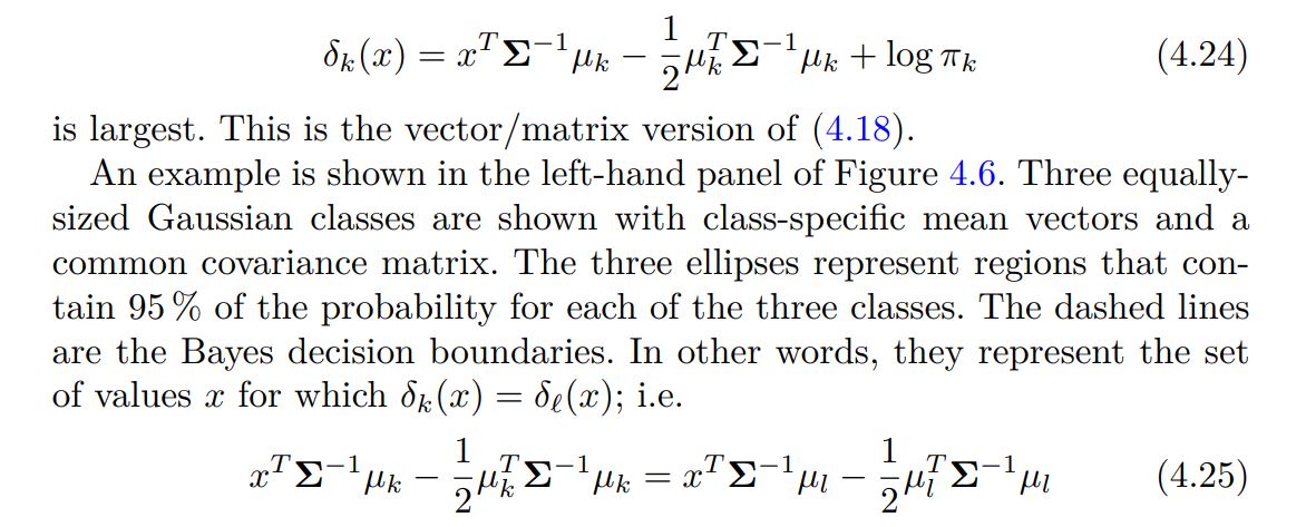
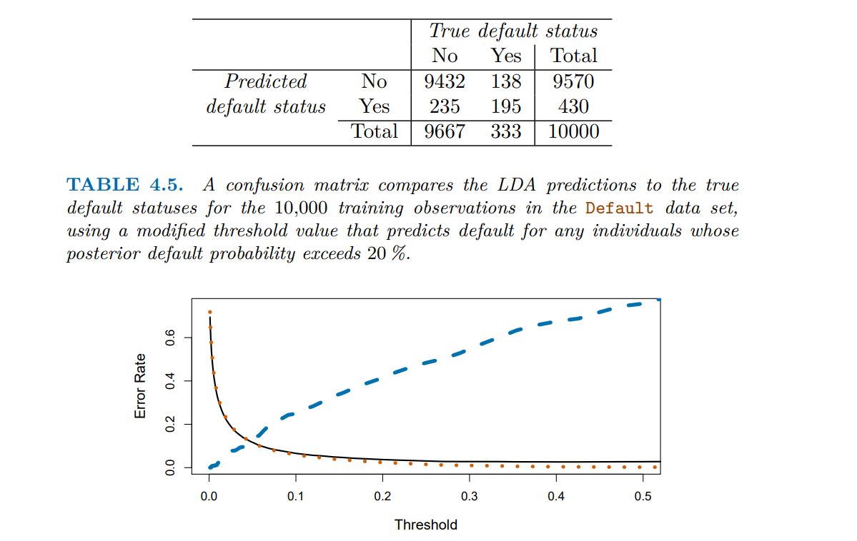
Result (confusion matrix)
ROC
The ROC curve is a popular graphic for simultaneously displaying the ROC curve two types of errors for all possible thresholds. The name “ROC” is historic, and comes from communications theory. It is an acronym for receiver operating characteristics. Figure 4.8 displays the ROC curve for the LDA classifier on the training data. The overall performance of a classifier, summarized over all possible thresholds, is given by the area under the (ROC) curve (AUC). An ideal ROC curve will hug the top left corner, so the larger the AUC the better the classifier. For this data the AUC is 0.95, which is close to the maximum of 1.0, so would be considered very good. We expect a classifier that performs no better than chance to have an AUC of 0.5 (when evaluated on an independent test set not used in model training). ROC curves are useful for comparing different classifiers, since they take into account all possible thresholds. It turns out that the ROC curve for the logistic regression model of Section 4.3.4 ft to these data is virtually indistinguishable from this one for the LDA model, so we do not display it here.
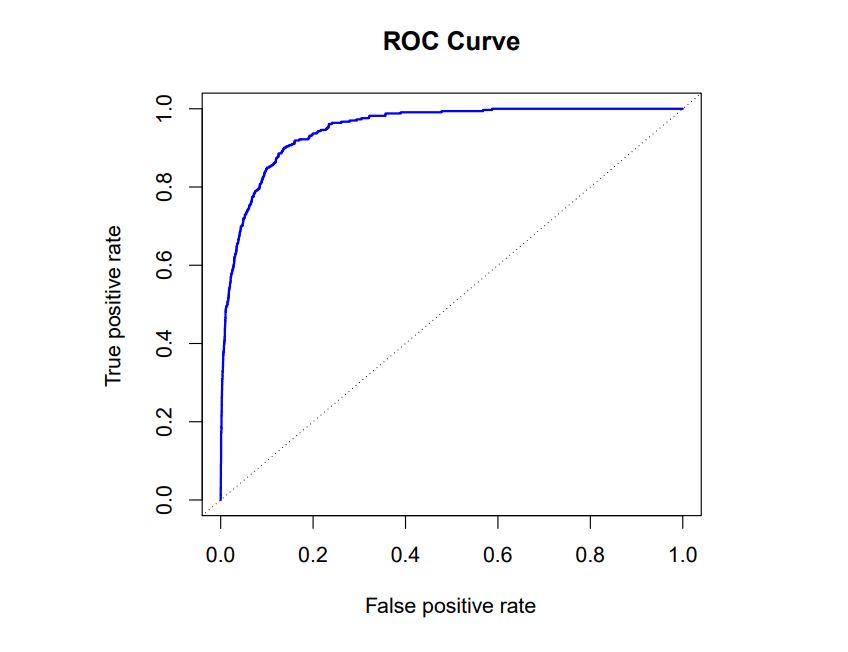
A ROC curve for the LDA classifier on the Default data. It traces out two types of error as we vary the threshold value for the posterior probability of default. The actual thresholds are not shown. The true positive rate is the sensitivity: the fraction of defaulters that are correctly identified, using a given threshold value. The false positive rate is 1-specifcity: the fraction of non-defaulters that we classify incorrectly as defaulters, using that same threshold value. The ideal ROC curve hugs the top left corner, indicating a high true positive rate and a low false positive rate. The dotted line represents the “no information” classifier; this is what we would expect if student status and credit card balance are not associated with probability of default.
------------------------------------------------------------------------
4.4.3 Quadratic Discriminant Analysis
------------------------------------------------------------------------
As we have discussed, LDA assumes that the observations within each class are drawn from a multivariate Gaussian distribution with a class-specifc mean vector and a covariance matrix that is common to all K classes. Quadratic discriminant analysis (QDA) provides an alternative approach Like LDA, the QDA classifier results from assuming that the observations from each class are drawn from a Gaussian distribution, and plugging estimates for the parameters into Bayes’ theorem in order to perform prediction. However, unlike LDA, QDA assumes that each class has its own covariance matrix. That is, it assumes that an observation from the kth class is of the form X ∼ N(µk, Σk), where Σk is a covariance matrix for the kth class. Under this assumption, the Bayes classifer assigns an observation X = x to the class for which is largest
As we have discussed, LDA assumes that the observations within each class are drawn from a multivariate Gaussian distribution with a class-specific mean vector and a covariance matrix that is common to all K classes. Quadratic discriminant analysis (QDA) provides an alternative approach Like LDA, the QDA classifier results from assuming that the observations from each class are drawn from a Gaussian distribution, and plugging estimates for the parameters into Bayes’ theorem in order to perform prediction. However, unlike LDA, QDA assumes that each class has its own covariance matrix. That is, it assumes that an observation from the kth class is of the form X ∼ N(µk, Σk), where Σk is a covariance matrix for the kth class. Under this assumption, the Bayes classifier assigns an observation X = x to the class is largest for which
------------------------------------------------------------------------
4.4.4 Naïve Bayes
------------------------------------------------------------------------
In previous sections, we used Bayes’ theorem to develop the LDA and QDA classifiers. Here, we use Bayes’ theorem to motivate the popular naïve Bayes classifier.
Recall that Bayes’ theorem provides an expression for the posterior probability pk(x) = Pr(Y = k|X = x) in terms of π1 .......... πk and f1(x) ..... fk(x). To use in practice, we need estimates for π1 .......... πk and f1(x) ..... fk(x). As we saw in previous sections, estimating the prior probabilities π1 .......... πk To use in practice, we need estimates for π1 .......... πk is typically straightforward: for instance, we can estimate ˆ&k as the proportion.
The naïve Bayes classifier takes a different tack for estimating f1(x), . . . , fK(x). Instead of assuming that these functions belong to a particular family of distributions (e.g. multivariate normal), we instead make a single assumption:
Within the kth class, the p predictors are independent.
Stated mathematically, this assumption means that for k = 1, . . . ,K,
$$f_{k}(x) = f_{k1}(x1) × f_{k2}(x2) × · · · × f_{kp}(xp),$$
where fkj is the density function of the jth predictor among observations in the kth class.
where Why is this assumption so powerful? Essentially, estimating a p-dimensional density function is challenging because we must consider not only the marginal distribution of each predictor that is, the distribution of each predictor on its own but also the joint distribution of the predictors that is, the association between the different predictors.
In the case of a multivariate normal distribution, the association between the different predictors is summarized by the off-diagonal elements of the covariance matrix. However, in general, this association can be very hard to characterize, and exceedingly challenging to estimate. But by assuming that the p covariates are independent within each class, we completely eliminate the need to worry about the association between the p predictors, because we have simply assumed that there is no association between the predictors!
4.5 A Comparison of Classification Methods
------------------------------------------------------------------------
4.5.1 An Analytical Comparison
------------------------------------------------------------------------
We now perform an analytical (or mathematical) comparison of LDA, QDA, naïve Bayes, and logistic regression. We consider these approaches in a setting with K classes, so that we assign an observation to the class that maximizes Pr(Y = k|X = x). Equivalently, we can set K as the baseline class and assign an observation to the class that maximizes

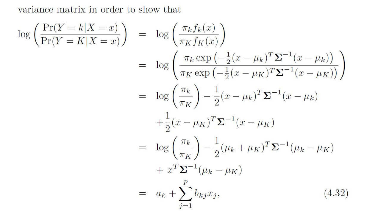
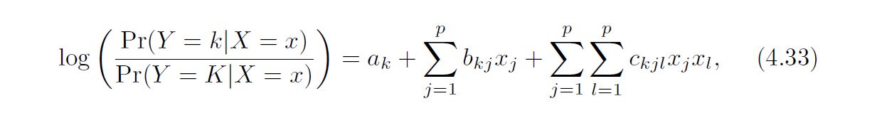
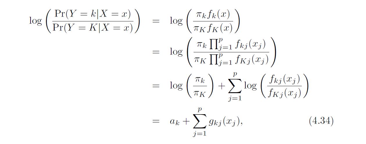
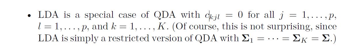
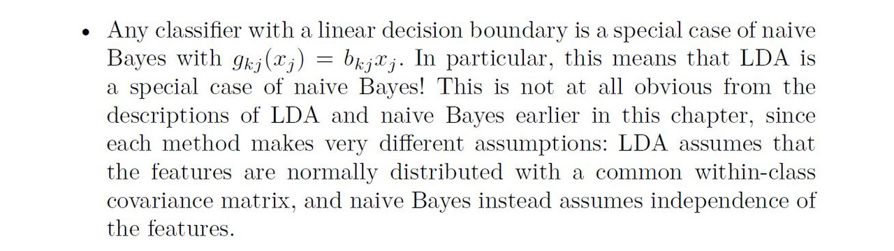
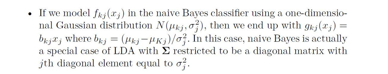
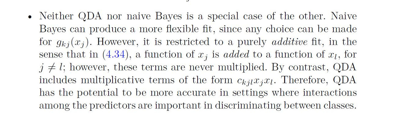
Inspection of (4.32), (4.33), and (4.34) yields the following observations about LDA, QDA, and naïve Bayes:
We close with a brief discussion of K-nearest neighbors (KNN). Recall that KNN takes a completely different approach from the classifiers seen in this chapter. In order to make a prediction for an observation X = x, the training observations that are closest to x are identified. Then X is assigned to the class to which the plurality of these observations belong. Hence KNN is a completely non-parametric approach: no assumptions are made about the shape of the decision boundary. We make the following observations about KNN:
------------------------------------------------------------------------
4.5.2 An Empirical Comparison
------------------------------------------------------------------------
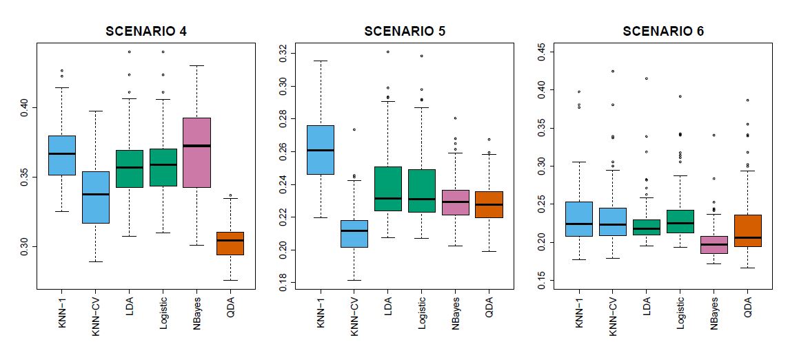
We now compare the empirical (practical) performance of logistic regression, LDA, QDA, naïve Bayes, and KNN. We generated data from six different scenarios, each of which involves a binary (two-class) classification problem. In three of the scenarios, the Bayes decision boundary is linear, and in the remaining scenarios it is non-linear. For each scenario, we produced 100 random training data sets. On each of these training sets, we fit each method to the data and computed the resulting test error rate on a large test set. Results for the linear scenarios are shown in Figure 4.11, and the results for the non-linear scenarios are in Figure 4.12. The KNN method requires selection of K, the number of neighbors (not to be confused with the number of classes in earlier sections of this chapter). We performed KNN with two values of K: K = 1, and a value of K that was chosen automatically using an approach called cross-validation, which we discuss further in Chapter 5. We applied naïve Bayes assuming univariate Gaussian densities for the features within each class (and, of course — since this is the key characteristic of naïve Bayes — assuming independence of the features). In each of the six scenarios, there were p = 2 quantitative predictors. The scenarios were as follows:
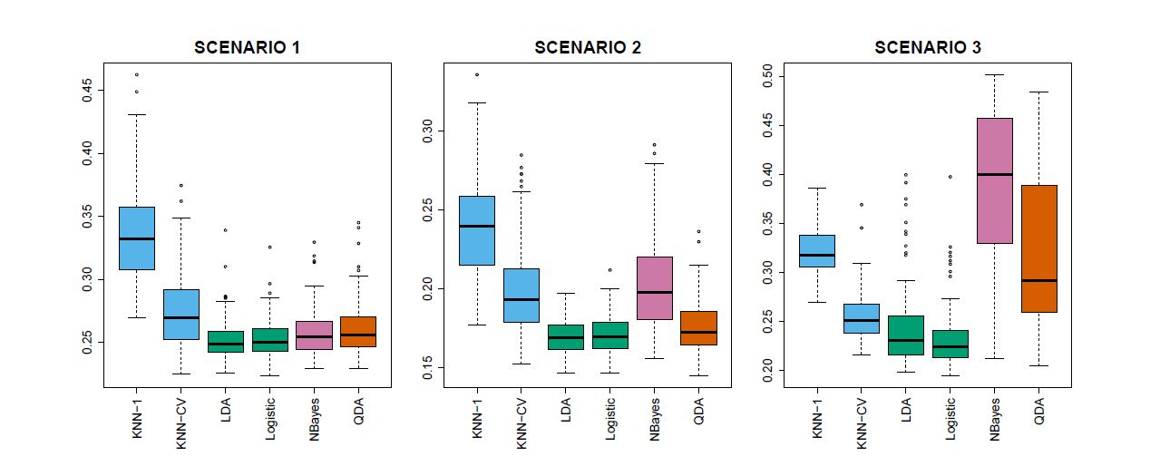
Scenario 1: There were 20 training observations in each of two classes. The observations within each class were uncorrelated random normal variables with a different mean in each class. The left-hand panel of Figure 4.11 shows that LDA performed well in this setting, as one would expect since this is the model assumed by LDA. Logistic regression also performed quite well, since it assumes a linear decision boundary. KNN performed poorly because it paid a price in terms of variance that was not offset by a reduction in bias. QDA also performed worse than LDA, since it fit a more flexible classifier than necessary. The performance of naïve Bayes was slightly better than QDA, because the naïve Bayes assumption of independent predictors is correct.
Scenario 2: Details are as in Scenario 1, except that within each class, the two predictors had a correlation of −0.5. The center panel of Figure 4.11 indicates that the performance of most methods is similar to the previous scenario. The notable exception is naïve Bayes, which performs very poorly here, since the naïve Bayes assumption of independent predictors is violated.
Scenario 3: As in the previous scenario, there is substantial negative correlation between the predictors within each class. However, this time we generated X1 and X2 from the t-distribution, with 50 observations per class. The t-distribution has a similar shape to the normal distribution, but it has a tendency to yield more extreme points—that is, more points that are far from the mean. In this setting, the decision boundary was still linear, and so fit into the logistic regression framework. The set-up violated the assumptions of LDA, since the observations were not drawn from a normal distribution. The right-hand panel of Figure 4.11 shows that logistic regression outperformed LDA, though both methods were superior to the other approaches. In particular, the QDA results deteriorated considerably as a consequence of non-normality. Naïve Bayes performed very poorly because the independence assumption is violated.
Scenario 4: The data were generated from a normal distribution, with a correlation of 0.5 between the predictors in the first class, and correlation of −0.5 between the predictors in the second class. This setup corresponded to the QDA assumption, and resulted in quadratic decision boundaries. The left-hand panel of Figure 4.12 shows that QDA outperformed all of the other approaches. The naïve Bayes assumption of independent predictors is violated, so naïve Bayes performs poorly.
Scenario 5: The data were generated from a normal distribution with uncorrelated predictors. Then the responses were sampled from the logistic function applied to a complicated non-linear function of the predictors. The center panel of Figure 4.12 shows that both QDA and naïve Bayes gave slightly better results than the linear methods, while the much more flexible KNN-CV method gave the best results. But KNN with K = 1 gave the worst results out of all methods. This highlights the fact that even when the data exhibits a complex non-linear relationship, a non-parametric method such as KNN can still give poor results if the level of smoothness is not chosen correctly.
Scenario 6: The observations were generated from a normal distribution with a different diagonal covariance matrix for each class. However, the sample size was very small: just n = 6 in each class. Naïve Bayes performed very well, because its assumptions are met. LDA and logistic regression performed poorly because the true decision boundary is non-linear, due to the unequal covariance matrices. QDA performed a bit worse than naïve Bayes, because given the very small sample size, the former incurred too much variance in estimating the correlation between the predictors within each class. KNN’s performance also suffered due to the very small sample size.
These six examples illustrate that no one method will dominate the others in every situation. When the true decision boundaries are linear, then the LDA and logistic regression approaches will tend to perform well. When the boundaries are moderately non-linear, QDA or naïve Bayes may give better results. Finally, for much more complicated decision boundaries, a non-parametric approach such as KNN can be superior. But the level of smoothness for a non-parametric approach must be chosen carefully. In the next chapter we examine a number of approaches for choosing the correct level of smoothness and, in general, for selecting the best overall method. Finally, recall from Chapter 3 that in the regression setting we can accommodate a non-linear relationship between the predictors and the response by performing regression using transformations of the predictors. A similar approach could be taken in the classification setting:
For instance, we could create a more flexible version of logistic regression by including X2, X3, and even X4 as predictors. This may or may not improve logistic regression’s performance, depending on whether the increase in variance due to the added flexibility is offset by a sufficiently large reduction in bias. We could do the same for LDA. If we added all possible quadratic terms and cross-products to LDA, the form of the model would be the same as the QDA model, although the parameter estimates would be different. This device allows us to move somewhere between an LDA and a QDA model.
------------------------------------------------------------------------
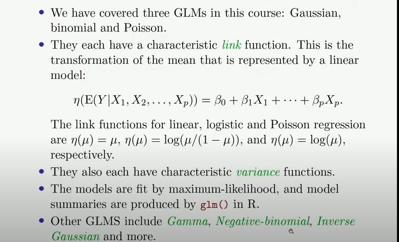
4.6 Generalized Linear Models
------------------------------------------------------------------------
In Chapter 3, we assumed that the response Y is quantitative, and explored the use of least squares linear regression to predict Y . Thus far in this chapter, we have instead assumed that Y is qualitative. However, we may sometimes be faced with situations in which Y is neither qualitative nor quantitative, and so neither linear regression from Chapter 3 nor the classification approaches covered in this chapter is applicable.
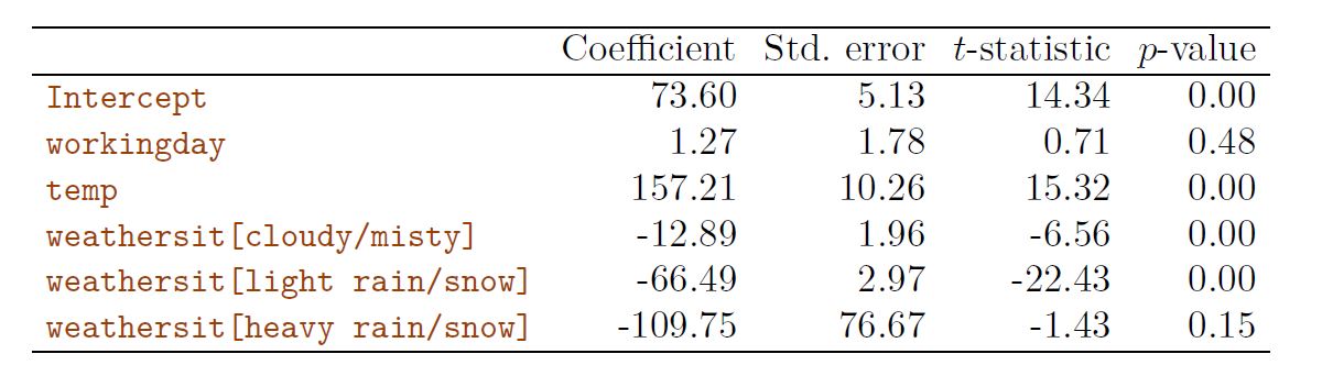
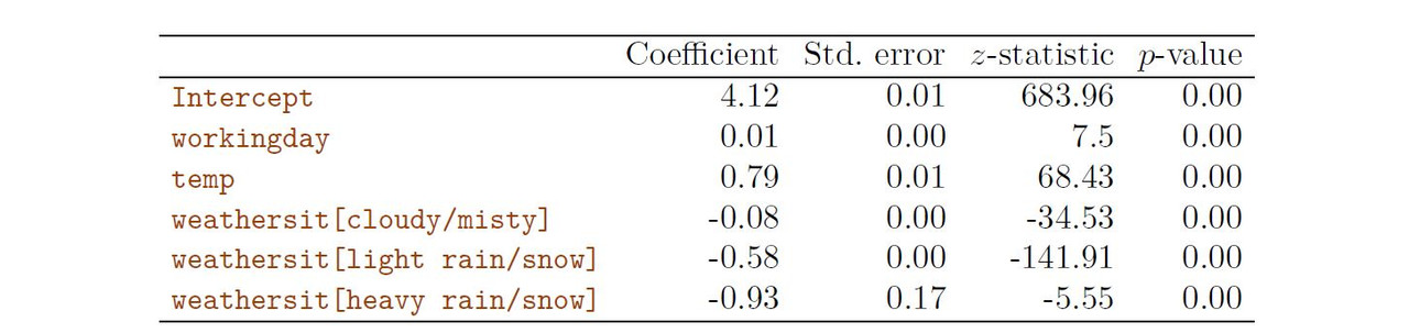
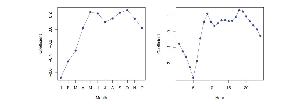
As a concrete example, we consider the Bikeshare data set. The response is bikers, the number of hourly users of a bike sharing program in Washington, DC. This response value is neither qualitative nor quantitative: instead, it takes on non-negative integer values, or counts. We will consider predicting bikers using the covariates month (month of the year), hr (hour of the day, from 0 to 23), working day (an indicator variable that equals 1 if it is neither a weekend nor a holiday), temp (the normalized temperature, in Celsius), and weather sit (a qualitative variable that takes on one of four possible values: clear; misty or cloudy; light rain or light snow; or heavy rain or heavy snow.) In the analyses that follow, we will treat (month), (hr), and (weather sit) as qualitative variables.
------------------------------------------------------------------------
4.6.1 Linear Regression on the Bikeshare Data
------------------------------------------------------------------------
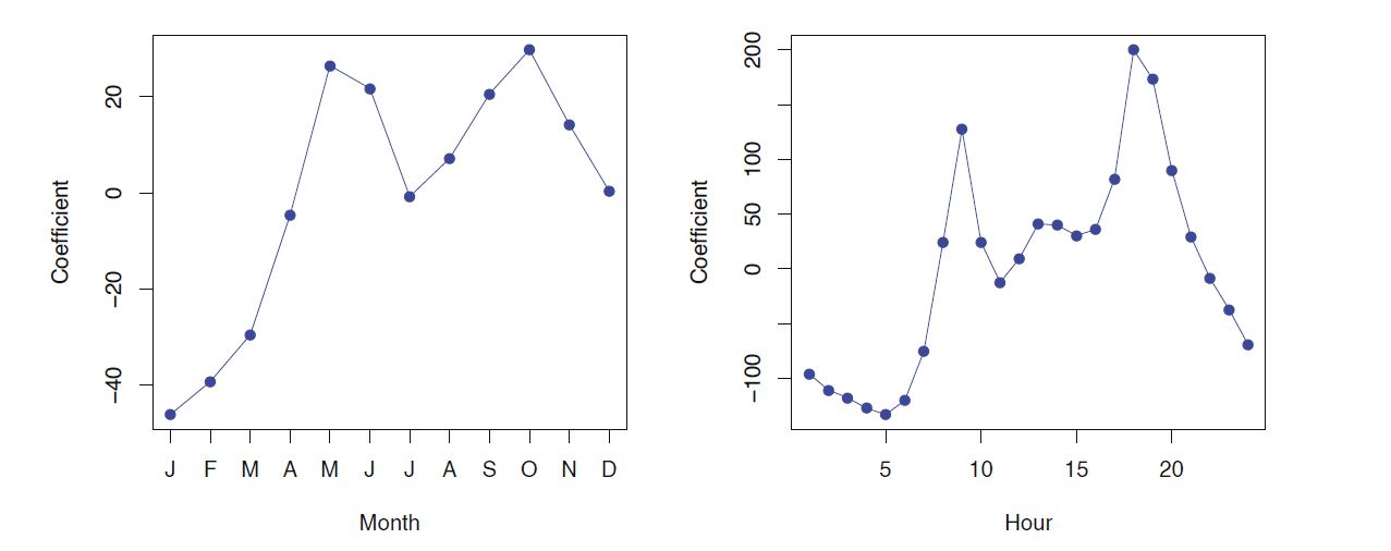
Results for a least squares linear model fit to predict bikers in the Bikeshare data.
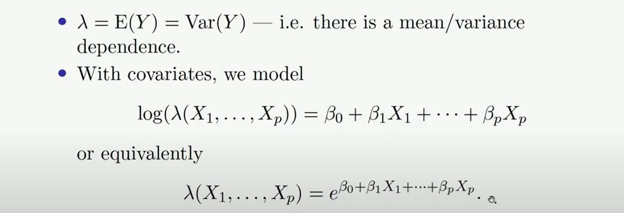
Mean/Variance Relationship
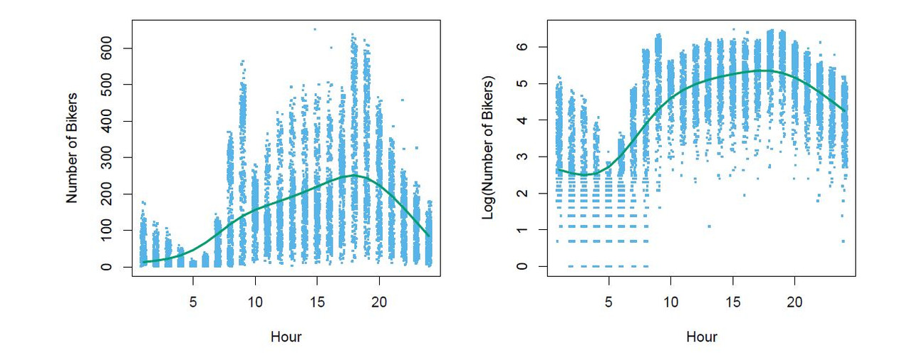
In the left plot we see that the variance mostly increase with the mean 10% of the linear model predictions are negative. (not shown here) Taking the log(Bikers) alleviates this, but has its own problems: e.g predictions are on the wrong scale and sum counts are zeros
------------------------------------------------------------------------
4.6.2 Poisson Regression on the Bikeshare Data
------------------------------------------------------------------------
Poisson Distribution is useful for modeling counts:

------------------------------------------------------------------------
4.6.3 Generalized Linear Models in Greater Generality
------------------------------------------------------------------------