Table of Content
7 Moving Beyond Linearity
The truth is never linear or almost never, but often the linearity assumption is good enough
When it is not ..... the following methods offers a lot of flexibility, without losing the ease and interpretability of linear models
Polynomial
Step functions
splines
Local regression
generalized additive models
Polynomial regression extends the linear model by adding extra predictors, obtained by raising each of the original predictors to a power. For example, a cubic regression uses three variables, X, X2, and X3, as predictors. This approach provides a simple way to provide a nonlinear fit to data.
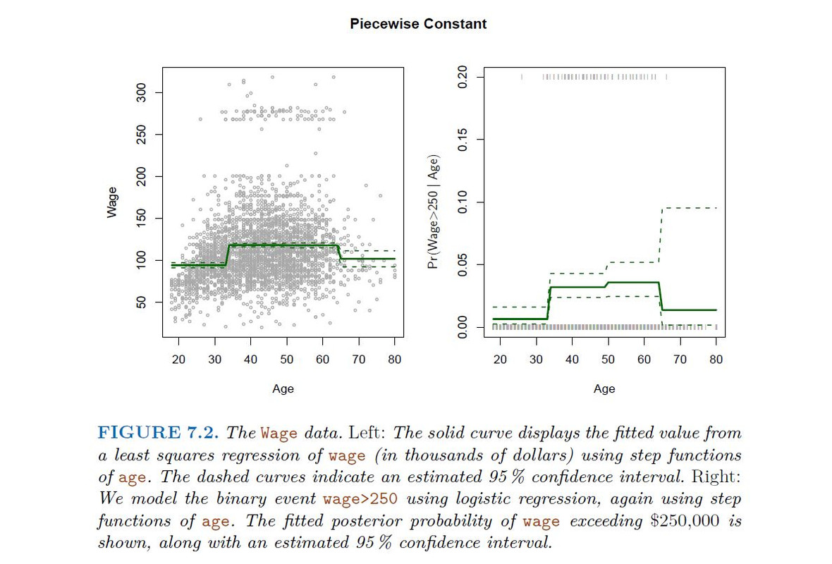
Step functions cut the range of a variable into K distinct regions in order to produce a qualitative variable. This has the effect of fitting a piecewise constant function.
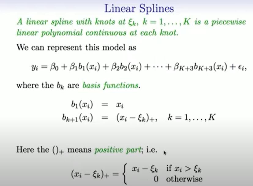
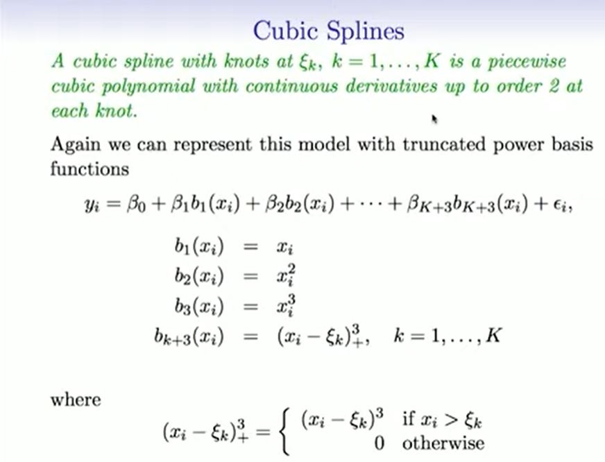
Regression splines are more flexible than polynomials and step functions, and in fact are an extension of the two. They involve dividing the range of X into K distinct regions. Within each region, a polynomial function is fit to the data. However, these polynomials are constrained so that they join smoothly at the region boundaries, or knots. Provided that the interval is divided into enough regions, this can produce an extremely flexible fit.
Smoothing splines are similar to regression splines, but arise in a slightly different situation. Smoothing splines result from minimizing a residual sum of squares criterion subject to a smoothness penalty.
Local regression is similar to splines, but differs in an important way. The regions are allowed to overlap, and indeed they do so in a very smooth way.
Generalized additive models allow us to extend the methods above to deal with multiple predictors.
-------------------------------------------------------
7.1 Polynomial Regression
-------------------------------------------------------
Historically, the standard way to extend linear regression to settings in which the relationship between the predictors and the response is nonlinear has been to replace the standard linear model
$$Y_{i} =B_{0} + B_{1} X_{i} + \epsilon$$
with a polynomial function
$$Y_{i} =B_{0} + B_{1} X_{i} + B_{2} X^2_{i} + B_{3} X^3_{i} + ..... + B_{d} X^d_{i} + \epsilon$$
where ϵ is the error term. This approach is known as polynomial regression,
The Details
Create new variables
$$X_{1}= X, X2 = X^2$$
, etc and then treat as multiple linear regression.
Not really interested in the coefficients; more interested in the fitted function values at any value X0:
$$\hat{f}(x_{0}) = \hat{B}_{0} + \hat{B}_{1}x_{0}+ \hat{B}_{2}x_{0}^2 + \hat{B}_{3}x_{0}^3+ \hat{B}_{4}x_{0}^4$$

We either fix the degree d at some reasonably low value, else use cross-calidation to choose d.
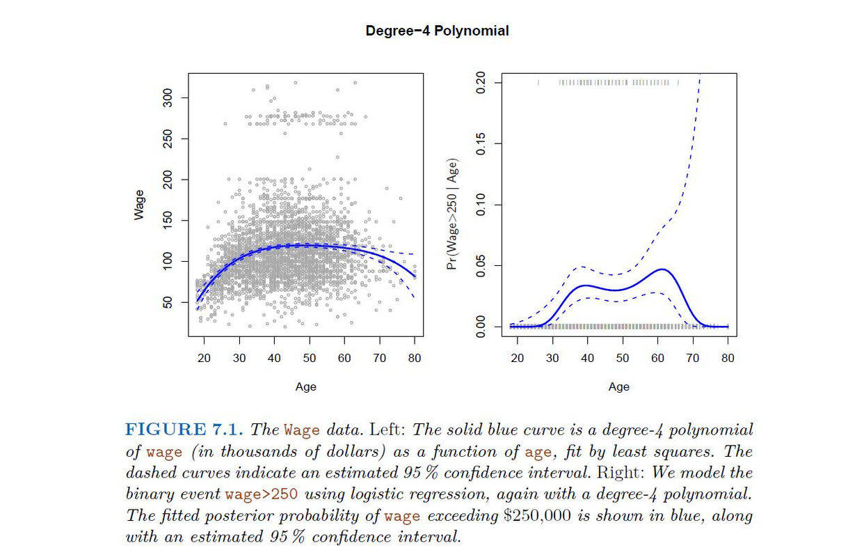
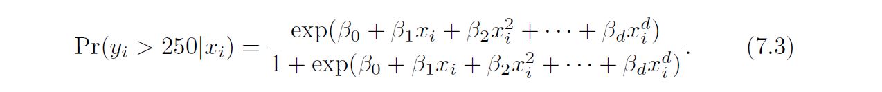
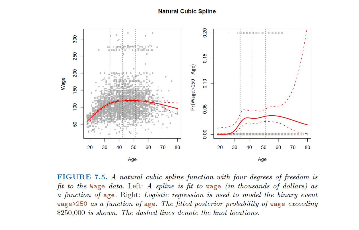
Logistic regression follows naturally. FOr example, in figure we model
To get confidence intervals, compute upper and lower bound on on the logit scale, and then invert to get on probability scale.
Can do separately on several variables just stack the variables into one matrix, and separate out the pieces afterwards (see GAMs later).
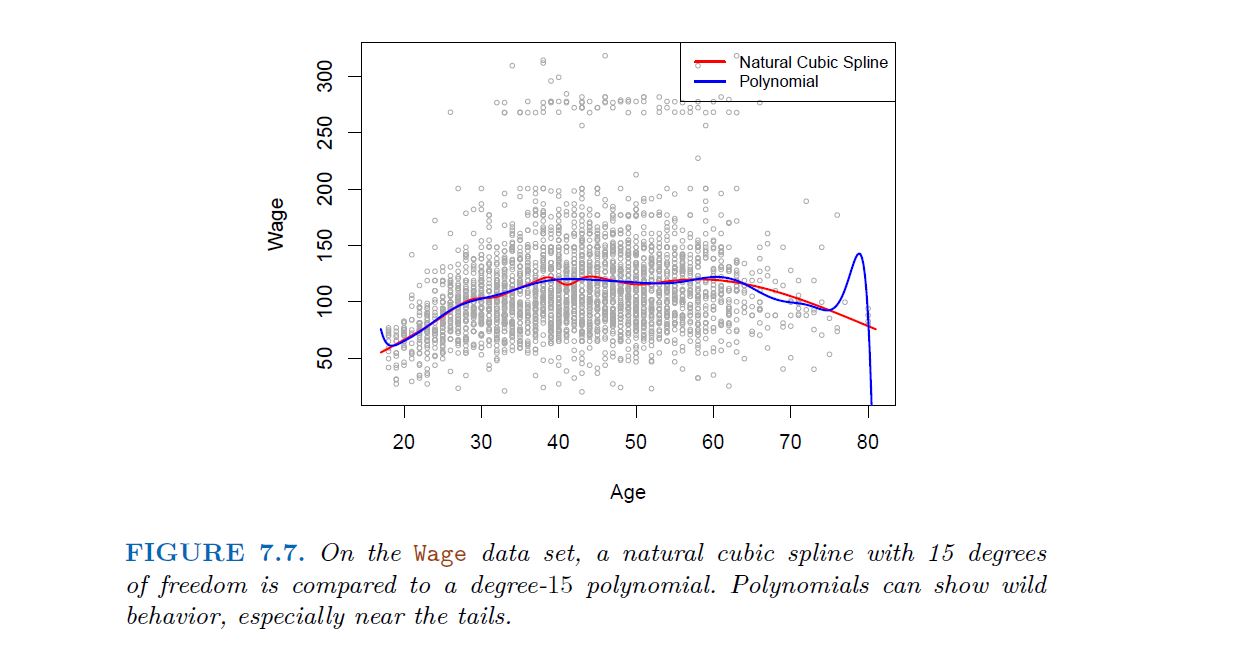
Caveat: polynomials have notorious tail behavior ـــــ Very bad for extrapolation.
Can fit using Y ~ poly(x, degree=3) in formula
-------------------------------------------------------
7.2 Step Functions
-------------------------------------------------------
Another way of creating transformation os a variable cut the variable into distinct regions
In greater detail, we create cut points c1, c2, . . . , cK in the range of X, and then construct K + 1 new variables
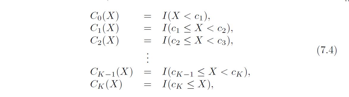
where I(·) is an indicator function that returns a 1 if the condition is true, indicator and returns a 0 otherwise. For example, I(cK <= X) equals 1 if cK <= X, and function equals 0 otherwise. These are sometimes called dummy variables. Notice that for any value of X, C0(X)+C1(X)+· · ·+CK(X) = 1, since X must be in exactly one of the K +1 intervals. We then use least squares to fit a linear model using C1(X), C2(X), . . . ,CK(X) as $predictors²
$$Y_{i} =B_{0} + B_{1} C_{1}(x_{i}) + B_{2} C_{2}(x_{i}) + ..... + B_{k} C_{k}(x_{i}) + \epsilon$$
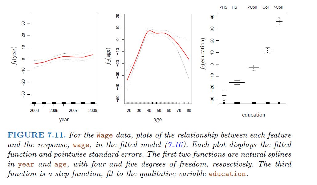
Step functions are easy to work with. Creates a series of dummy variables representing each group. Useful way of creating interactions that are easy to interpret. For example interaction effect of year and age: I(year<2005).Age, I(year>=2005).Age would allow for different linear functions in each age category Choice of cut points or knots can be problematic. For creating nonlinearities, smoother alternatives such as splines are available
-------------------------------------------------------
7.3 Basis Functions
-------------------------------------------------------
Polynomial and piecewise-constant regression models are in fact special cases of a basis function approach. The idea is to have at hand a family of functions or transformations that can be applied to a variable X: b1(X), b2(X), . . . , bK(X). Instead of fitting a linear model in X, we fit the model

-------------------------------------------------------
7.4 Regression Splines
-------------------------------------------------------
Now we discuss a flexible class of basis functions that extends upon the polynomial regression and piecewise constant regression approaches that we have just seen.
-------------------------------------------------------
7.4.1 Piecewise Polynomials
-------------------------------------------------------
Instead of a single polynomial in X over its whole domain, we can rather use different polynomials in regions defined by knots

Better to add constraints to the polynomials, e.g. continuity. Splines have the "maximum" amount of continuity
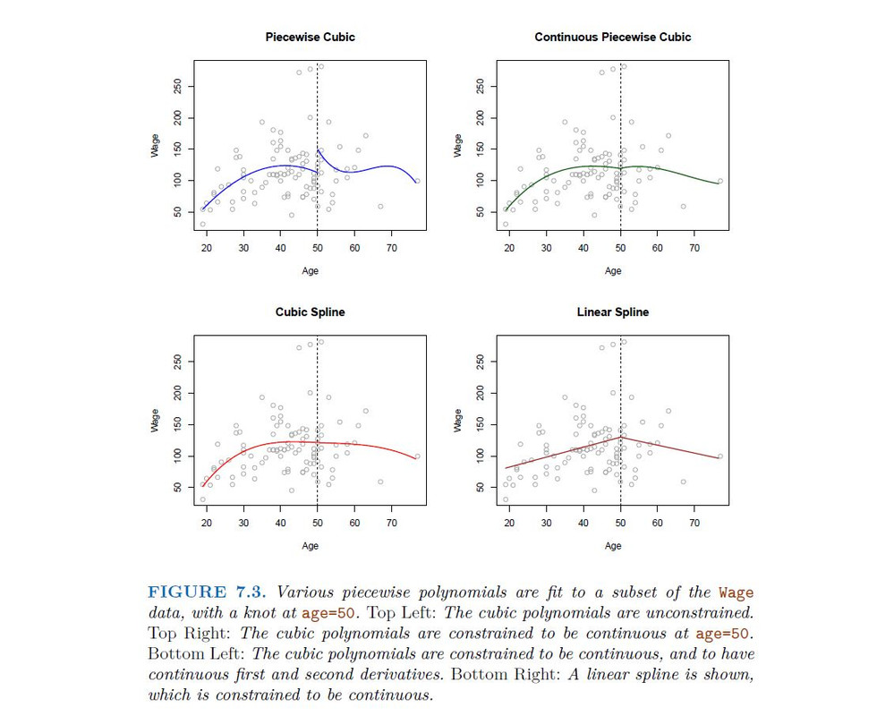
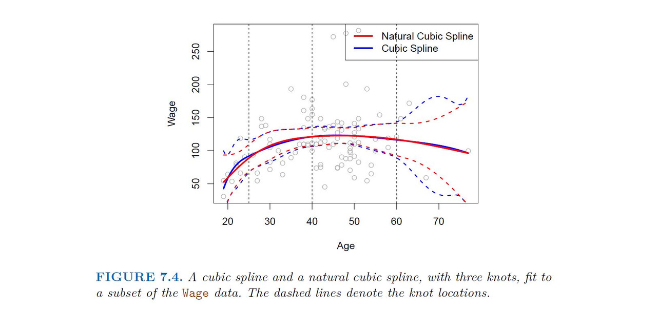
Natural Cubic Spline
A natural cubic spline extrapolates linearity beyond the boundary knots. This adds 4 = 2 * 2 extra constraints, and allows us to put more internal knots fir the same degrees of freedom as a regular cubic spline
-------------------------------------------------------
7.4.2 Choosing the Number and Locations of the Knots
-------------------------------------------------------
When we fit a spline, where should we place the knots? The regression spline is most flexible in regions that contain a lot of knots, because in those regions the polynomial coefficients can change rapidly. Hence, one option is to place more knots in places where we feel the function might vary most rapidly, and to place fewer knots where it seems more stable. While this option can work well, in practice it is common to place knots in a uniform fashion. One way to do this is to specify the desired degrees of freedom, and then have the software automatically place the corresponding number of knots at uniform quantiles of the data.
knot Placement
One strategy is to decide K, the number of knots, and then place them at appropriate quantiles of the observed X.
A cubic spline with K nots has K + 4 parameters or degrees of freedom.
A natural spline with K nots has K degrees of freedom.
-------------------------------------------------------
7.5 Smoothing Splines
-------------------------------------------------------
In the last section we discussed regression splines, which we create by specifying a set of knots, producing a sequence of basis functions, and then using least squares to estimate the spline coefficients. We now introduce a somewhat different approach that also produces a spline.
-------------------------------------------------------
7.5.1 An Overview of Smoothing Splines
-------------------------------------------------------
In fitting a smooth curve to a set of data, what we really want to do is find some function, say g(x), that fits the observed data well: that is, we want
$$RSS = \sum_{i=1}^{n} (y_{i} - g(x_{i}))^2$$
to be small. However, there is a problem with this approach. If we don’t put any constraints on g(xi), then we can always make RSS zero simply by choosing g such that it interpolates all of the yi. Such a function would woefully overfit the data—it would be far too flexible. What we really want is a function g that makes RSS small, but that is also smooth.
but that is also smooth. How might we ensure that g is smooth? There are a number of ways to do this. A natural approach is to find the function g that minimizes
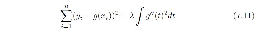
where λ is a nonnegative tuning parameter. The function g that minimizes (7.11) is known as a smoothing spline.
The first term is RSS, and tires to make g(x) match the data at Xi The second term is a roughness penalty and controls how wiggly g(x) is. It is modulated by the tuning parameter λ >= 0. The smaller λ, the more wiggly that the function, eventually interpolating yi
$$when \ λ = 0 \ As \ λ \ \rightarrow \infty, \ the \ function \ g(x) \ becomes\ linear$$
-------------------------------------------------------
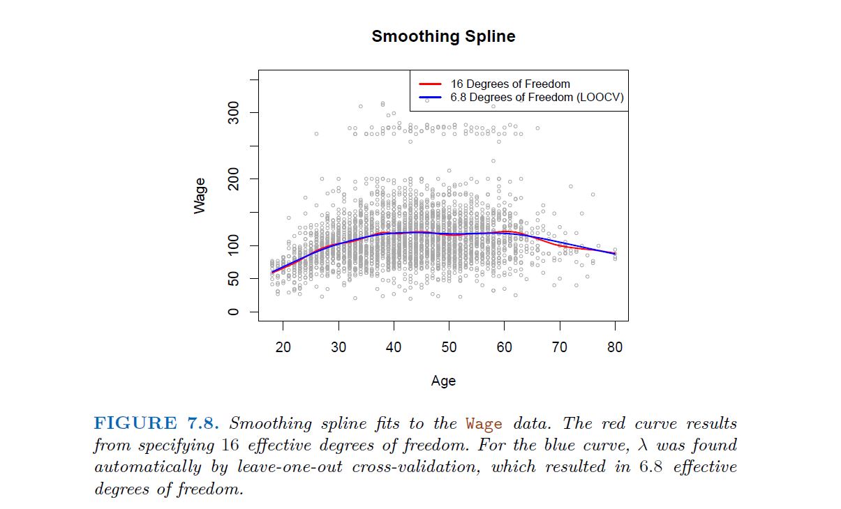
7.5.2 Choosing the Smoothing Parameter $\lambda$
-------------------------------------------------------
The solution is a natural cubic spline, with knot at every unique value of $x_{i}$. The roughness penalty still controls the roughness via $\lambda$
Some details
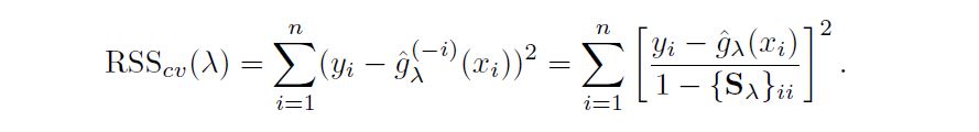
Smoothing splines avoid the knot-selection issue, leaving a single $\lambda$ to be chosen. The algorithmic details are too complex to describe here. in R, the function smooth.spline() will fit a smoothing spline. In Python (spline = UnivariateSpline(x, y, s=1)) The vector of n fitted values can be written as $\hat{g}_{\lambda}$ = $S_{\lambda}Y$, where $S_{\lambda}$ is a n * n matrix (determined by the $x_{i}$ and $\lambda$) The effective degrees of freedom are given by:

In fitting a smoothing spline, we do not need to select the number or location of the knots—there will be a knot at each training observation, x1, . . . ,xn. Instead, we have another problem: we need to choose the value of $\lambda$ The leave-one-out (LOO) cross-validated error is given by
-------------------------------------------------------
7.6 Local Regression
-------------------------------------------------------
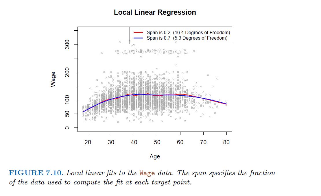
Local regression is a different approach for fitting flexible non-linear functions, which involves computing the fit at a target point $x_{0}$ using only the nearby training observations.
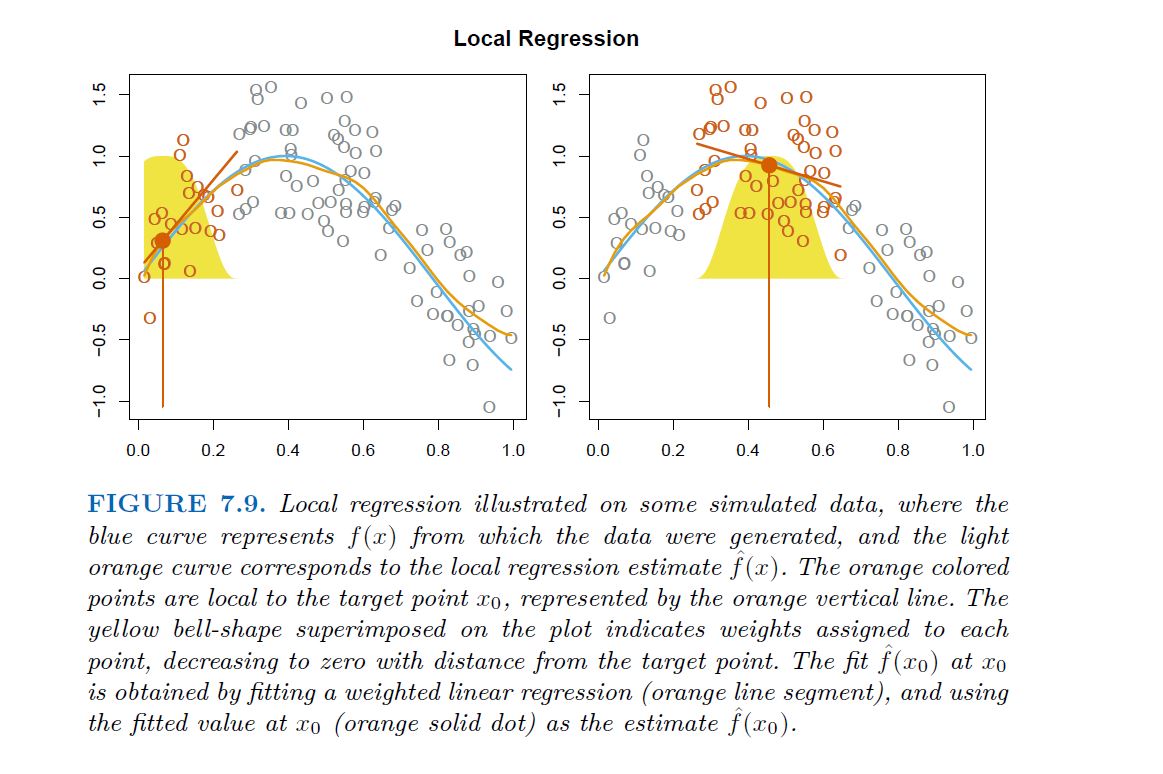
Algorithm 7.1 Local Regression At X =x0
Gather the fraction s = k/n of training points whose xi are closest to x0.
Assign a weight Kio = K(xi, x0) to each point in this neighborhood, so that the point furthest from x0 has weight zero, and the closest has the highest weight. All but these k nearest neighbors get weight zero.
Fit a weighted least squares regression of the yi on the xi using the aforementioned weights, by finding B^0 and B^1 that minimize.
The fitted value at x0 is given by
$$\hat{f}(x_{0}) = \hat{B}_{0} + \hat{B}_{1}x_{0}$$
-------------------------------------------------------
7.7 Generalized Additive Models
-------------------------------------------------------
Allows for flexible nonlinearities in several variables, but retains the additive structure of linear models
$$Y_{i} =B_{0} + f_{1}(x_{i1}) + f_{2}(x_{i2}) + ..... + f_{p}(x_{ip})+ \epsilon_{i}$$