


Table of Content
6. Linear Model Selection and Regularization
Why might we want to use another fitting procedure instead of least squares?
As we will see, alternative fitting procedures can yield better prediction accuracy and model interpretability.
Prediction Accuracy: Provided that the true relationship between the response and the predictors is approximately linear, the least squares estimates will have low bias. If n + p—that is, if n, the number of observations, is much larger than p, the number of variables—then the least squares estimates tend to also have low variance, and hence will perform well on test observations. However, if n is not much larger than p, then there can be a lot of variability in the least squares fit, resulting in overfitting and consequently poor predictions on future observations not used in model training. And if p > n, then there is no longer a unique least squares coefficient estimate: there are infinitely many solutions. Each of these least squares solutions gives zero error on the training data, but typically very poor test set performance due to extremely high variance.1 By constraining or shrinking the estimated coefficients, we can often substantially reduce the variance at the cost of a negligible increase in bias. This can lead to substantial improvements in the accuracy with which we can predict the response for observations not used in model training.
Model Interpretability: It is often the case that some or many of the variables used in a multiple regression model are in fact not associated with the response. Including such irrelevant variables leads to unnecessary complexity in the resulting model. By removing these variables—that is, by setting the corresponding coefficient estimates to zero—we can obtain a model that is more easily interpreted. Now least squares is extremely unlikely to yield any coefficient estimates that are exactly zero. In this chapter, we see some approaches for automatically performing feature selection or variable selection that is for excluding irrelevant variables from a multiple regression model.
There are many alternatives, both classical and modern, to using least squares to fit (6.1). In this chapter, we discuss three important classes of methods.
Subset Selection: This approach involves identifying a subset of the p predictors that we believe to be related to the response. We then fit a model using least squares on the reduced set of variables. Shrinkage: This approach involves fitting a model involving all p predictors. However, the estimated coefficients are shrunken towards zero relative to the least squares estimates. This shrinkage (also known as regularization) has the effect of reducing variance. Depending on what type of shrinkage is performed, some of the coefficients may be estimated to be exactly zero. Hence, shrinkage methods can also perform variable selection. Dimension Reduction: This approach involves projecting the p predictors into an M-dimensional subspace, where M < P. This is achieved by computing M different linear combinations, or projections, of the variables. Then these M projections are used as predictors to fit a linear regression model by least squares.
6.1 Subset Selection
-----------------------------------------------------
6.1.1 Best Subset Selection
-----------------------------------------------------
To perform best subset selection, we fit a separate least squares regression for each possible combination of the p predictors That is, we fit all p models that contain exactly one predictor, all
$$\binom{p}{2} = \frac{p(p - 1)}{2}$$
models that contain exactly two predictors, and so forth. We then look at all of the resulting models, with the goal of identifying the one that is best.
Best subset selection Algorithm
Let M0 denote the null model, which contains no predictors. This model simply predicts the sample mean for each observation.
For k = 1, 2, . . .p: Fit all
$$\binom{p}{k}$$
models that contain exactly k predictors
Pick the best among these
$$\binom{p}{k}$$
models, and call it Mk Here best is defined as having the smallest RSS, or equivalently largest R².
Select a single best model from among M0, . . . ,Mp using the prediction error on a validation set, Cp (AIC), BIC, or adjusted R².
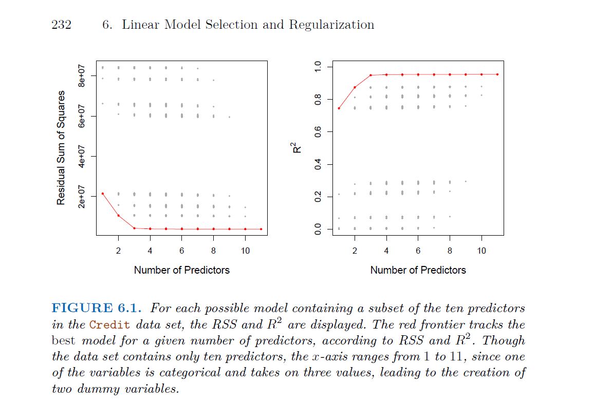
Now in order to select a single best model, we must simply choose among these p + 1 options. This task must be performed with care, because the RSS of these p + 1 models decreases monotonically, and the R2 increases monotonically, as the number of features included in the models increases. Therefore, if we use these statistics to select the best model, then we will always end up with a model involving all of the variables. The problem is that a low RSS or a high R2 indicates a model with a low training error, whereas we wish to choose a model that has a low test error.
As illustrated in the graph on the left, several models with two predictors are displayed, with the one marked by the red line representing the best-performing model. Similarly, the best models for those with 3, 4, and 5 predictors are also highlighted. However, it is important to note that the performance of models with two predictors cannot be directly compared to those with three or more predictors.
While best subset selection is a simple and conceptually appealing approach, it suffers from computational limitations. The number of possible models that must be considered grows rapidly as p increases. In general, there are 2p models that involve subsets of p predictors. So if p = 10, then there are approximately 1,000 possible models to be considered, and if p = 20, then there are over one million possibilities! Consequently, best subset selection becomes computationally infeasible for values of p greater than around 40, even with extremely fast modern computers. There are computational shortcuts so called branch-and-bound techniques for eliminating some choices, but these have their limitations as p gets large. They also only work for least squares linear regression. We present computationally efficient alternatives to best subset selection next.
-----------------------------------------------------
6.1.2 Stepwise Selection
-----------------------------------------------------
For computational reasons, best subset selection cannot be applied with very large p. Best subset selection may also suffer from statistical problems when p is large. The larger the search space, the higher the chance of finding models that look good on the training data, even though they might not have any predictive power on future data. Thus an enormous search space can lead to overfitting and high variance of the coefficient estimates. For both of these reasons, stepwise methods, which explore a far more restricted set of models, are attractive alternatives to best subset selection.
Forward stepwise selection is a computationally efficient alternative to best subset selection. While the best subset selection procedure considers all $2^{p}$ possible models containing subsets of the p predictors, forward stepwise considers a much smaller set of models. Forward stepwise selection begins with a model containing no predictors, and then adds predictors to the model, one-at-a-time, until all of the predictors are in the model. In particular, at each step the variable that gives the greatest additional improvement to the fit is added to the model. More formally, the forward stepwise selection procedure is given in Algorithm 6.2
Forward Stepwise Selection Algorithm
Forward stepwise selection beings with a model containing no predictors, and then adds predictors to the model, one-at-a-time until all of the predictors are in the model In particular, at each at each step the variable that gives the greatest additional improvement to the fit is added to the model.
Let M0 denote the null model, which contains no predictors. For k = 0, . . .p-1: Consider all p − k models that augment the predictors in Mk with one additional predictor. Choose the best among these p − k models, and call it Mk+1. Here best is defined as having smallest RSS or highest R². Select a single best model from among M0, . . . ,Mp using the prediction error on a validation set, Cp (AIC), BIC, or adjusted R². Or use the cross-validation method.
Computational advantages over best subset selection is clear. It is not guaranteed to find the best possible model out of all 2^p models containing subset of the p predictors.

Backward Stepwise Selection Algorithm
Like forward stepwise selection, backward stepwise selection provides an efficient alternative to best subset selection. However, unlike forward stepwise selection, it begins with the full least squares model containing all p predictors, and then iteratively removes the least useful predictor, one-at a- time.
Let Mp denote the full model, which contains all p predictors. For k = p,p-1 . . .,1: Consider all k models that contain all but one of the predictors in Mk for a total of k − 1 predictors. Choose the best among these k models, and call it Mk - 1. Here best is defined as having smallest RSS or highest $R^2$. Select a single best model from among M0, . . . Mp using the prediction error on a validation set, Cp (AIC), BIC, or adjusted R². Or use the cross-validation method.
Like forward stepwise selection, the backward selection approach searches through only 1+p(p+1)/2 models, and so can be applied in settings where p is too large to apply best subset selection. like forward stepwise selection, backward stepwise selection is not guaranteed to yield the best model containing a subset of the p predictors. Backward selection requires that the number of samples n is larger than the number of variables p (so that the full model can be fit). In contrast, forward stepwise can be used even when n < p, and so is the only viable subset method when p is very large.
Hybrid Approaches
The best subset, forward stepwise, and backward stepwise selection approaches generally give similar but not identical models. As another alternative, hybrid versions of forward and backward stepwise selection are available, in which variables are added to the model sequentially, in analogy to forward selection. However, after adding each new variable, the method may also remove any variables that no longer provide an improvement in the model fit. Such an approach attempts to more closely mimic best subset selection while retaining the computational advantages of forward and backward stepwise selection.
-----------------------------------------------------
6.1.3 Choosing the Optimal Model
-----------------------------------------------------
The model containing all of the predictors will always have the smallest RSS and the largest R³ , since these quantities are related to the training error. We wish to choose a model with low test error not a model with low training error. Recall that training error is usually a poor estimate of the test error Therefore, RSS and R² are not suitable for selecting the best model among a collection of models with different numbers of predictions
Best subset selection, forward selection, and backward selection result in the creation of a set of models, each of which contains a subset of the p predictors. To apply these methods, we need a way to determine which of these models is best
Estimating Test Error
There are two common approaches:
We can indirectly estimate test error by making an adjustment to the training error to account for the bias due to overfitting. We can directly estimate the test error, using either a validation set approach or a cross-validation approach.
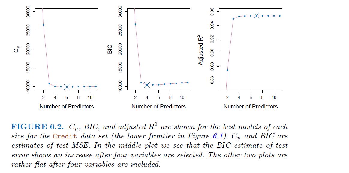
Cp, AIC, BIC, and Adjusted R²
These techniques adjust the training error for the model size, and can be used to select among a set of models with different numbers of variables. The next figure displays Cp, BIC and adjusted R² for the best model of each size produced by best subset selection on the credit data set

Validation and Cross-Validation
As an alternative to the approaches just discussed, we can directly estimate the test error using the validation set and cross-validation methods.
We can compute the validation set error or the cross-validation error for each model under consideration, and then select the model for which the resulting estimated test error is smallest.
Each of the procedures returns a sequence of models $M_{k}$ indexed by model size k= 0,1,2,3,...... Our job here is to select K^. Once selected, we will return model $M_\hat{k}$ We compute the validation set error or the cross-validation error for each model Mk under confederation, and then select the k for which the resulting estimated test error is smallest. This procedure has an advantage relative to AIC, BIC, Cp and adjusted R², in that it provides a direct estimate of the test error, and doesn't require an estimate of the error variance σ²
-----------------------------------------------------
6.2 Shrinkage Methods
-----------------------------------------------------
The subset selection methods involve using least squares to fit a linear model that contains a subset of the predictors. As an alternative, we can fit a model containing all p predictors using a technique that constrains or regularizes the coefficient estimates, or equivalently, that shrinks the coefficient estimates towards zero. It may not be immediately obvious why such a constraint should improve the fit, but it turns out that shrinking the coefficient estimates can significantly reduce their variance. The two best-known techniques for shrinking the regression coefficients towards zero are ridge regression and the lasso.
-----------------------------------------------------
6.2.1 Ridge Regression
-----------------------------------------------------
Recall from Chapter 3 that the least squares fitting procedure estimates B0, B1, . . . , Bp using the values that minimize

Ridge regression is very similar to least squares, except that the coefficients are estimated by minimizing a slightly different quantity. In particular, the ridge regression coefficient estimates (B^)**R are the values that minimize
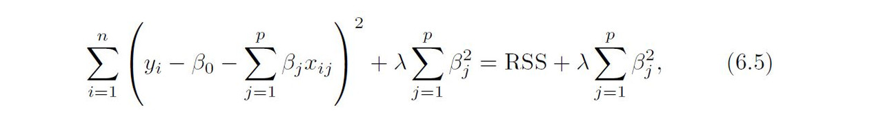
Where λ >= 0 is a tuning parameter, to be determined separately
Ridge regression: scaling of predictors
The standard least squares coefficient estimates are scale equivariant: multiplying Xj by a constant c simply leads to a scaling of the least squares coefficient estimates by a factor of 1/c. In other words, regardless of how the jth predictor is scaled,
$$X_{j}\hat{B}_{j}$$
will remain the same.
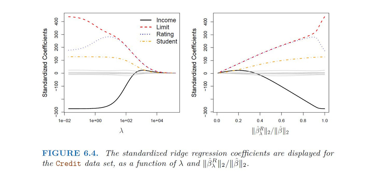
In contrast, the ridge regression coefficient estimates can change substantially when a given predictor is multiplied by a constant, due to the sum of squared coefficients term in the penalty part of the ridge regression objective function.
Therefore, it is best to apply ridge regression after standardizing the predictors using the formula

-----------------------------------------------------
6.2.2 The Lasso
-----------------------------------------------------
Ridge regression does have one obvious disadvantage. Unlike best subset, which will generally select models that involve just a subset of the variables, ridge regression will include all p predictors in the final model.
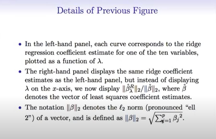
The lasso is a relatively recent alternative to ridge regression that over- comes this disadvantage. The lasso coefficients, $\hat{B}_{\lambda}^L$, minimize the quantity

the lasso uses an ℓ1 (pronounced “ell 1”) penalty instead of an ℓ2 penalty. The ℓ1 norm of a coefficient vector B is given by
$$||B||{1} = \sum|B{j}|$$
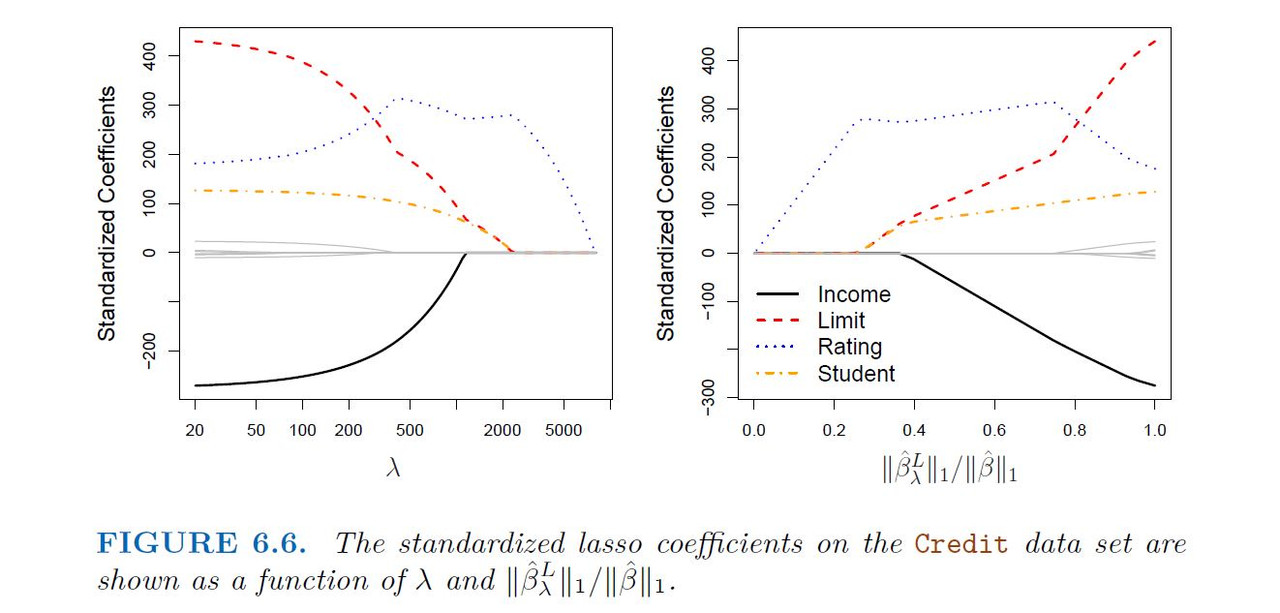
As with ridge regression, the lasso shrinks the coefficient estimates towards zero. However, in the case of the lasso, the ℓ1 penalty has the effect of forcing some of the coefficient estimates to be exactly equal to zero when the tuning parameter ! is sufficiently large Hence, much like best subset selection,the lasso performs variable selection. We say that the lasso yields sparse models that is, sparse models that involve only a subset of the variables. As in ridge regression, selecting a good value of $\lambda$ for the lasso is critical; cross-validation is again the method of choice.
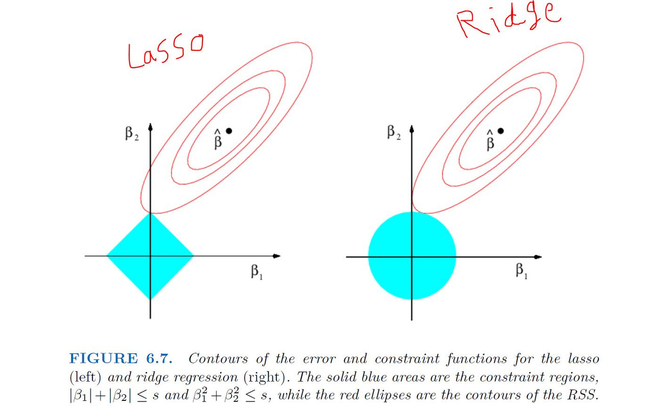
The Variable Selection Property of the Lasso
Why is it that the lasso, unlike ridge regression, results in coefficient estimates that are exactly equal to zero?
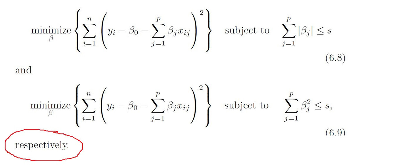
One can show that the lasso and the ridge regression coefficient estimates solve the problems
Comparing the Lasso and Ridge Regression

Conclusion
These tow examples illustrate that neither ridge regression nor the lasso will universally dominate other. In general, one might expect the lasso to perform better when response is a function of only a relatively small number of the predictors. However, the number of predictors that is related to the response is never known a prior for real data sets. A technique such as cross-validation can be used in order to determine which approach is better on a particular data set
Selecting the Tuning Parameter for Ridge and Lasso
Just as the subset selection, for Ridge and lasso require a method to determine which of the models under consideration is best That is, We requires a method for selecting a value for the tuning parameter $\lambda$ or equivalently, the value of constraint s Cross-validation provides a simple way to tackle this problem. We choose a grid of λ values, and compute the cross-validation error for each value of λ. We then select the tuning parameter value for which the cross-validation error is smallest. Finally, the model is re-fit using all of the available observations and the selected value of the tuning parameter.
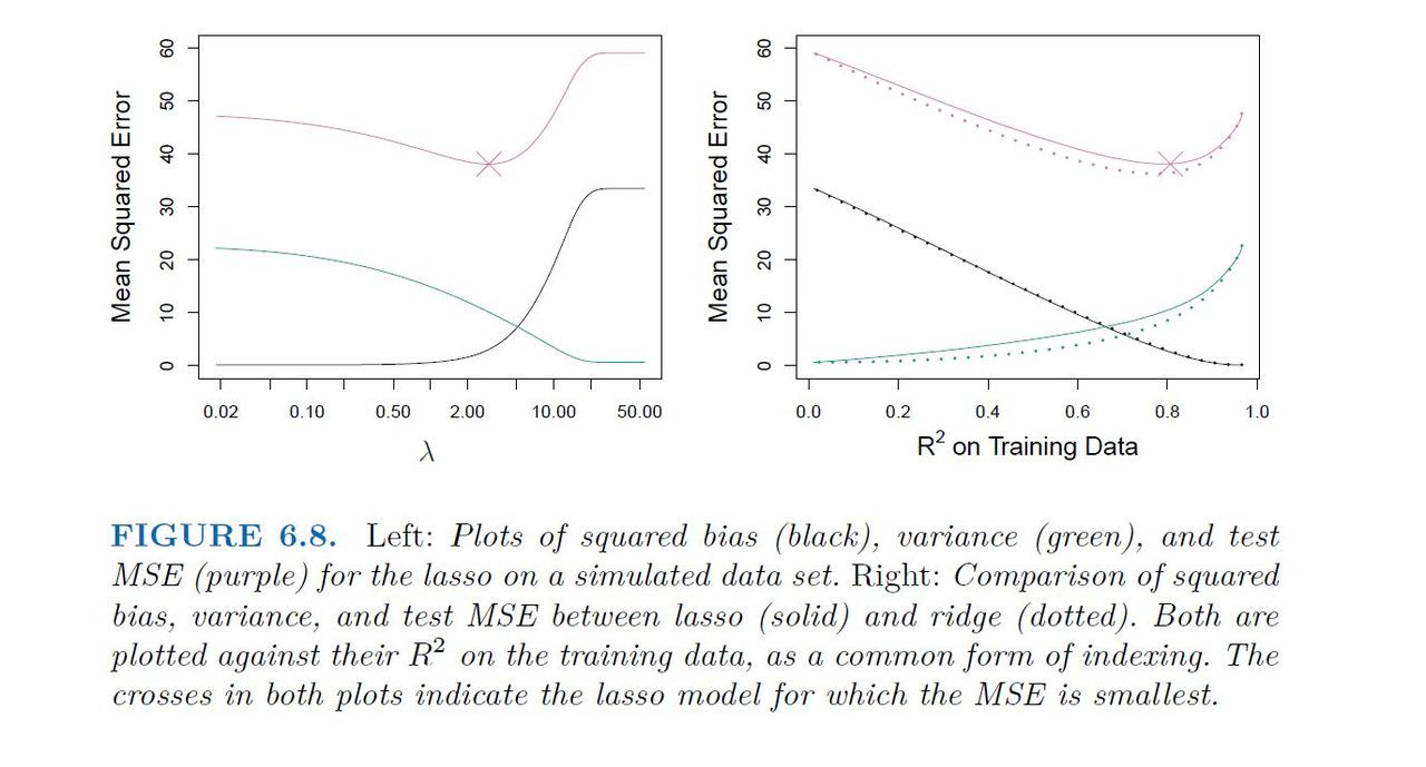
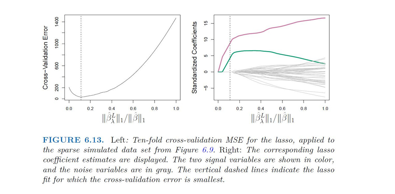
Simulated Data Example
-----------------------------------------------------
6.3 Dimension Reduction Methods
-----------------------------------------------------
The methods that we have discussed so far in this chapter have controlled variance in two different ways, either by using a subset of the original variables, or by shrinking their coefficients toward zero. All of these methods are defined using the original predictors, X1,X2, . . . ,Xp We now explore a class of approaches that transform the predictors and then fit a least squares model using the transformed variables. We will refer to these techniques as dimension reduction methods. Let Z1, Z2, . . . ,Zm represent M < p linear combinations of our original p predictors. That is,
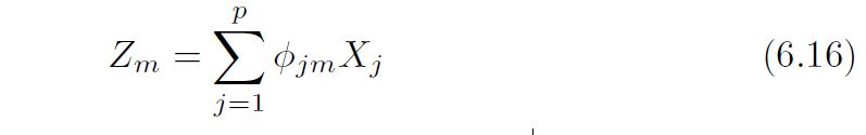
for some constants ϕ1m, ϕ2m . . . , ϕpm, m = 1, . . . ,M. We can then fit the linear regression model (using least squares.)

Note that in model(2), the regression coefficients are given by θ0, θ1, .... θm If the constants ϕ1m, ϕ2m . . . , ϕpm are chosen wisely, then such dimension reduction approaches can often outperform least squares regression. Notice that from 6.16
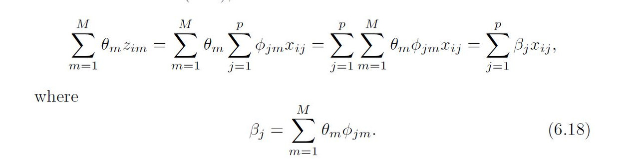
Hence (6.17) can be thought of as a special case of the original linear regression model Dimension reduction serves to constrain the estimated Bj coefficients, since now they must take the form (6.18). Can win in bias-variance tradeoff
Note that this is only going to work nicely if M>P
-----------------------------------------------------
6.3.1 Principal Components Regression
-----------------------------------------------------
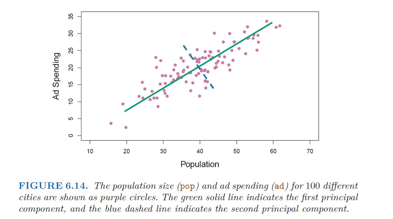
Principal components analysis (PCA) is a popular approach for deriving a low-dimensional set of features from a large set of variables.
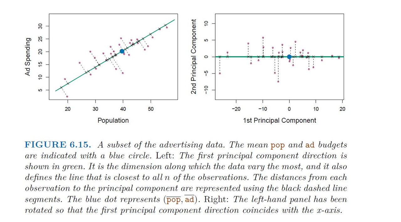
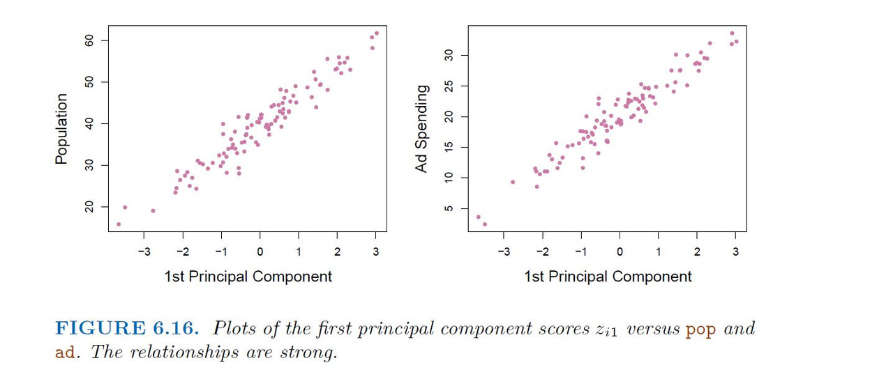
PCA is a technique for reducing the dimension of an n*p data matrix X. The first principal component direction of the data is that along which the observations vary the most.
Example
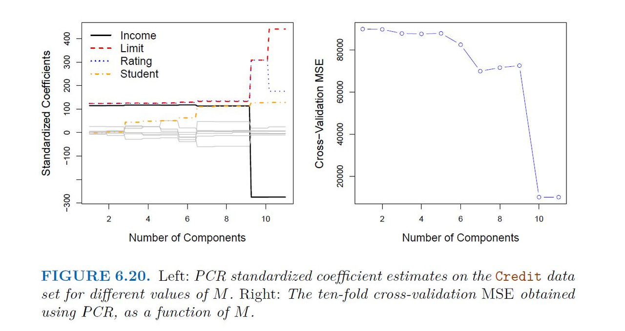
Application of Principal Components Regression
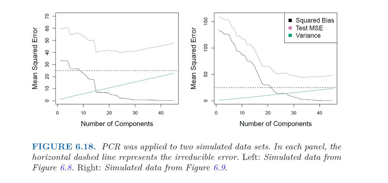
Choosing the number of directions
-----------------------------------------------------
6.3.2 Partial Least Squares
-----------------------------------------------------
The PCR approach that we just described involves identifying linear combinations, or directions, that best represent the predictors X1, . . . , Xp.
These directions are identified in an unsupervised way, since the response Y is not used to help determine the principal component directions. That is, the response does not supervise the identification of the principal components.
Consequently, PCR suffers from a drawback: there is no guarantee that the directions that best explain the predictors will also be the best directions to use for predicting the response.
Like PCR, PLS is a dimension reduction method, which first identifies new set of features Z1, . . . ,Zm that are linear combinations of the original features, and then fits a linear model via least squares using these M new features.
But unlike PCR, PLS identifies these new features in a supervised way that is, it makes use of the response Y in order to identify new features that not only approximate the old features well, but also that are related to the response.
Roughly speaking, the PLS approach attempts to find directions that help explain both the response and the predictors.
After standardizing the p predictors, PLS computes the first direction Z1 by setting each ϕj1 in (6.16) equal to the coefficient from the simple linear regression of Y onto Xj
One can show that this coefficient is proportional to the correlation between Y and Xj
Hence, in computing
$$Z_{1} = \sum^p_{j= 1} \phi_{j1} X_{j}$$
PLS places the highest weight on the variables that are most strongly related to the response.
Subsequent directions are found by taking residuals and then repeating the above prescription
Summary
Model selection methods are an essential tool for data analysis, especially for big datasets involving many predictors.
Research into methods that give sparsity, such as the Lasso is an especially hot area.
Later, we will return to sparsity in more details, and will describe related approaches such as the elastic net