


Table of Content
3. Linear Regression
Linear regression analysis allows us to investigate several key relationships between variables.
Here are a few important questions that we might seek to address (Examples)
1. Is there a relationship between advertising budget and sales?
2. How strong is the relationship between advertising budget and sales?
3. Which media are associated with sales?
4. How large is the association between each medium and sales?
5. How accurately can we predict future sales?
6. Is the relationship linear?
7. Is there synergy among (
interaction effect) the advertising media?
----------------------------------------------------------------------------------
3.1 Simple Linear Regression
----------------------------------------------------------------------------------
Simple linear regression lives up to its name: it is a very straightforward simple linear approach for predicting a quantitative response Y on the basis of a single predictor variable X. It assumes that there is approximately a linear relationship between X and Y. Mathematically, we can write this linear relationship as
$$Y \approx \beta_{0} + \beta_{1}X$$
𝑌: This represents the outcome or the dependent variable. It's what you are trying to predict or explain.
β0: This is the intercept. It's a constant term that represents the value of 𝑌 when 𝑋 is zero. Think of it as the starting point or baseline value of 𝑌
β1 : This is the slope or the coefficient for 𝑋. It tells you how much 𝑌 changes when 𝑋 changes by one unit. It's a measure of the relationship between 𝑋 and 𝑌.
Example
$$\text{Sales} \approx \beta_{0} + \beta_{1} \text{TV}$$
Once we have used our training data to produce estimates $\hat{β_{0}}$ and $\hat{β_{1}}$ for the model coefficients, we can predict future sales on the basis of a particular value of TV advertising by computing
$$\hat{y} ≈ \hat{β_{0}} + \hat{β_{1}}x$$
$$\hat{y}: indicates \ a \ prediction \ of\ Y.$$
----------------------------------------------------------------------------------
3.1.1 Estimating the Coefficients
----------------------------------------------------------------------------------
Residual Sum of Squares (RSS)
RSS stands for Residual Sum of Squares. It's a measure used in statistics and data analysis to assess the goodness of fit of a regression model. Let's break it down in simple terms.
What is RSS?
- Residual: The difference between the actual value and the predicted value from a regression model.
$$\text{Residual} = \text{Actual Value} - \text{Predicted Value}$$
- Sum of Squares: Squaring the residuals ensures they are all positive (since squaring a negative number makes it positive) and gives more weight to larger differences. The sum of these squared residuals across all data points is the RSS.
$$\text{RSS} = \sum (\text{Actual Value} - \text{Predicted Value})^2$$
3. Why is RSS Important?
Measure of Fit: RSS indicates how well your regression model fits the data. A lower RSS means a better fit because the model's predictions are closer to the actual values.
Model Comparison: When comparing different models, the one with the lower RSS is generally preferred, as it has less error in its predictions.
Example
Imagine you have a simple dataset with actual values of ( Y ) and predictions from your model:
| Data Point | Actual Value (( Y )) | Predicted Value Y^ | Residual (Y- Y^) | Squared Residual (Y- Y^)**2 |
| 1 | 10 | 8 | 2 | 4 |
| 2 | 15 | 14 | 1 | 1 |
| 3 | 14 | 12 | 2 | 4 |
| 4 | 12 | 10 | 2 | 4 |
To calculate the RSS:
Compute the residuals for each data point.
Square each residual.
Sum up all the squared residuals.
For this example:
RSS = 4 + 1 + 4 + 4 = 13
Summary
RSS quantifies the error of a regression model.
Lower RSS indicates a model that better fits the data.
It is used for evaluating and comparing different regression models.
Our Target to make RSS as small as possible
----------------------------------------------------------------------------------
3.1.2 Assessing the Accuracy of the Coefficient Estimates
----------------------------------------------------------------------------------
$$Y = β_{0} + β_{1}X$$
This linear regression equation assumes a perfect linear relationship without any error.
$$Y = β_{0} + β_{1}X + \epsilon$$
ϵ: Error term (the difference between the observed value and the value predicted by the model).
The second linear regression equation is more realistic for most real-world applications, where data typically exhibit some level of randomness and variability that the model cannot capture perfectly
The presence of the error term allows for statistical inference, such as hypothesis testing and confidence interval estimation for the coefficients.
Population Mean µ vs. Sample Mean µ^
$$ȳ = \hat{µ}$$
Imagine you want to know the average height (population mean, µ) of all the people in a city. But you can't measure everyone's height, so you measure the heights of 100 people (your sample).
Population Mean (µ): The true average height of everyone in the city.
Sample Mean (ȳ): The average height of the 100 people you measured.
The sample mean (ȳ) is a good estimate of the population mean (µ). While they are not the same, the sample mean gives us a reasonable idea of what the population mean might be.
Unbiased Estimators
An estimator is unbiased if, on average, it hits the true value. For example:
If we take many different samples and calculate the sample mean (ȳ) for each one, the average of all these sample means will be very close to the population mean (µ). This makes ȳ an unbiased estimator of µ.
Similarly, the estimates β^0 and β^1 are unbiased for the true coefficients β0 and β1. If we took many different samples and calculatedβ^0 and β^1 each time, the average of these estimates would be very close to the true β0 and β1
Standard Error
The standard error (SE) tells us how much the sample mean (ȳ) or is likely to vary from the population mean (µ). It gives us an idea of the accuracy of our estimate.
If the SE is small, our sample mean is likely to be close to the population mean.
If the SE is large, our sample mean might be far from the population mean.
Variance and Standard Error
Variance of the Estimate of the Mean ( $\hat{µ}$) and Its Standard Error:
$$Var(\hat{\mu}) = SE(\hat{\mu})^2 = \frac{\sigma^2}{n}$$
σ: The standard deviation of the actual Y Values.
n: The number of observations (data points).
SE(𝜇^): The standard error of the estimated mean (𝜇^), which tells us how much 𝜇^ is expected to vary from the actual mean (𝜇).
Residual Standard Error (RSE)
When we perform linear regression, we estimate the coefficients (intercept and slope). We want to know how close these estimates β^0 and β^1 are to the true values β0 and β1. To measure this, we use the standard errors (SE) of the estimates.
Since σ² or SE is often unknown, it is estimated from the data. This estimate is known as the residual standard error (RSE):
$$RSE = \sqrt{RSS / (n-2)}$$
Confidence Intervals
Standard errors can be used to compute confidence intervals. A 95% confidence interval gives a range of values within which we expect the true parameter value to lie with 95% probability.
Confidence Intervals for β1
$$\hat{B_{1}} ± 2.SE(\hat{B_{1}})$$
There is approximately a 95% chance that the following interval will contain the true value of β1
$$\hat{B_{1}} + 2.SE(\hat{B_{1}}) , \hat{B_{1}} - 2.SE(\hat{B_{1}})$$
Confidence Intervals for β0
$$\hat{B_{0}} ± 2.SE(\hat{B_{0}})$$
There is approximately a 95% chance that the following interval will contain the true value of β0
$$\hat{B_{0}} + 2.SE(\hat{B_{0}}) , \hat{B_{0}} - 2.SE(\hat{B_{0}})$$
In the case of the advertising data, the 95% confidence interval for β0 is [6.130 , 7.935] and the 95% confidence interval for β1 is [0.042 , 0.053]
Therefore, we can conclude that in the absence of any advertising, sales will, on average, fall somewhere between 6,130 and 7,935 units.(When X is 0 Intercept)
Furthermore, for each $1,000 increase in television advertising, there will be an average increase in sales of between 42 and 53 units.
Hypothesis Testing
Standard errors can also be used to perform hypothesis tests on the coefficients. The most common hypothesis test involves testing the null hypothesis of
$$H_{0}: \ There \ is \ no \ relationship \ between \ X \ and \ Y$$
versus the alternative hypothesis
$$H_{a}: \ There \ is \ some \ relationship \ between \ X \ and \ Y$$
Mathematically, this corresponds to testing
$$H_{0}: B_{1}=0$$
versus
$$H_{a}: B_{1} \neq 0$$
if β1 =0 then Y = β1 + ϵ and X is not associated with Y
To test the null hypothesis, we need to determine whether β^1, our estimate for β1, is sufficiently far from zero that we can be confident that β1 is non-zero.
How far is far enough?
This of course depends on the accuracy of β^1 which depends on SE(β^1).
if SE(β^1) is small, then even relatively small values of β^1 may provide strong evidence that β^1 ≠ 0, and hence that there is a relationship between X and Y.
In contrast, if SE(β^1) is large, then β^1 must be large in absolute value in order for us to reject the null hypothesis. In practice, we compute a t-statistic, t-statistic given by
$$t = \frac{\hat{B_1} - 0}{SE(\hat{B_1})}$$
| Predictor | Coefficient | Std. Error | t-statistic | p-value |
| Intercept | 7.0325 | 0.4578 | 15.36 | <0.0001 |
| TV | 0.0475 | 0.0027 | 17.67 | <0.0001 |
From above Results We can see that
1. Intercept
Coefficient ( β0 )
7.0325: This means that the expected value of the dependent variable (Sales) is 7.0325 when all predictor variables are zero. (When TV Advertising = 0)Std. Error
0.4578: This is the standard error of the intercept term. (smaller standard error indicates more precise estimates of the coefficient)t-statistic
15.36: This is the t-value from t-statistics test (It is used to test whether a coefficient is significantly different from zero to reject the null hypothesis)p-value
<0.0001: This very small p-value indicates that the intercept term is highly significant.
2. TV
Coefficient ( β1 )
0.0475: This means that for each additional unit of TV advertising, the Sales is expected to increase by 0.0475 units, holding other variables constant.Std. Error
0.0027: This is the standard error of the intercept term. (smaller standard error indicates more precise estimates of the coefficient)t-statistic
17.67: This is the t-value from t-statistics test (It is used to test whether a coefficient is significantly different from zero to reject the null hypothesis)p-value
<0.0001: This very small p-value indicates that the intercept term is highly significant.
t-statistics is large and p-value is Small which suggest that there is a correlation between TV advertising and sales
Notice that the coefficients for β^0 and β^1 are very large relative to their standard errors, so the t-statistics are also large; the probabilities of seeing such values if H0 is true are virtually zero. Hence we can conclude β0 ≠ 0 and β1 ≠ 0
----------------------------------------------------------------------------------
3.1.3 Assessing the Accuracy of the Model
----------------------------------------------------------------------------------
Once we have rejected the null hypothesis H0 in favor of the alternative hypothesis Ha, it is natural to want to quantify the extent to which the model fits the data. The quality of a linear regression fit is typically assessed using two related quantities: the residual standard error RSE and the R2 statistic
| Quantity | Value |
| Residual standard error | 3.26 |
| R² | 0.612 |
| F-statistic | 312.1 |
From above Results We can see that
RSE is 3.26. This means that on average, the observed values deviate from the predicted values by about 3.26 units. A smaller RSE indicates a better fit of the model to the data.
R² of 0.612 means that 61.2% of the variability in the dependent variable can be explained by the independent variables in the model. The closer the R² is to 1, the better the model explains the variability of the dependent variable. In this context, an R² of 0.612 indicates a moderately strong relationship between the predictors and the response variable.
F-statistic of 312.1 is quite high, indicating that the model is statistically significant. A high F-statistic suggests that the model provides a better fit to the data than a model with no predictors. The corresponding p-value would confirm the overall significance of the model..
Residual Standard Error (RSE): is a measure of the quality of a linear regression fit. It represents the average amount by which the observed values differ from the values predicted by the model.
R-squared( R² ) : is the proportion of the variance in the dependent variable that is predictable from the independent variables. It ranges from 0 to 1.
F-Statistic: measures the overall significance of the regression model. It tests whether at least one of the predictor variables has a non-zero coefficient.
----------------------------------------------------------------------------------
3.2 Multiple Linear Regression
----------------------------------------------------------------------------------
Simple linear regression is a useful approach for predicting a response on the basis of a single predictor variable. However, in practice we often have more than one predictor. However, the approach of fitting a separate simple linear regression model for each predictor is not entirely satisfactory.
Instead of fitting a separate simple linear regression model for each predictor, a better approach is to extend the simple linear regression model so it can directly accommodate multiple predictors. We can do this by giving each predictor a separate slope coefficient in a single model. In general, suppose that we have p distinct predictors. Then the multiple linear regression model takes the form
$$Y =B_{0} + B_{1} X_{1} + B_{2} X_{2} + ..... + + B_{p} X_{p} + \epsilon$$
for Example:
$$sales = B_{0} + B_{1} TV + B_{2} radio + B_{3} * newspaper + \epsilon.$$
-------------------------------------------------------------------------------------------------------------------------
3.2.1 Estimating the Regression Coefficients
-------------------------------------------------------------------------------------------------------------------------
Multiple Linear Regression
| Predictor | Coefficient | Std. Error | t-statistic | p-value |
| Intercept | 2.939 | 0.3119 | 9.42 | <0.0001 |
| TV | 0.046 | 0.0014 | 32.81 | <0.0001 |
| radio | 0.189 | 0.0086 | 21.89 | <0.0001 |
| newspaper | 0.001 | 0.0059 | 0.18 | 0.8599 |
From above Results We can see that
1. Intercept
Coefficient ( β0 )
2.939: This means that the expected value of the dependent variable (Sales) is 2.939 when all predictor variables are zero. (TV Advertising, Radio Advertising and Newspaper Advertising = 0)Std. Error
0.3119: This is the standard error of the intercept term. (smaller standard error indicates more precise estimates of the coefficient)t-statistic
9.42: This is the t-value from t-statistics test (It is used to test whether a coefficient is significantly different from zero to reject the null hypothesis)p-value
<0.0001: This very small p-value indicates that the intercept term is highly significant.
2. TV
Coefficient ( β1 )
0.046: This means that for each additional unit of TV advertising, the Sales is expected to increase by 0.046 units, holding other variables constant.Std. Error
0.0014: This is the standard error of the intercept term. (smaller standard error indicates more precise estimates of the coefficient)t-statistic
32.81: This is the t-value from t-statistics test (It is used to test whether a coefficient is significantly different from zero to reject the null hypothesis)p-value
<0.0001: This very small p-value indicates that the intercept term is highly significant.
t-statistics is large and p-value is Small which suggest that there is a correlation between TV advertising and sales
3. Radio
Coefficient ( β1 )
0.189: This means that for each additional unit of Radio advertising, the Sales is expected to increase by 0.189 units, holding other variables constant.Std. Error
0.0086: This is the standard error of the intercept term. (smaller standard error indicates more precise estimates of the coefficient)statistic
21.89: This is the t-value from t-statistics test (It is used to test whether a coefficient is significantly different from zero to reject the null hypothesis)p-value
<0.0001: This very small p-value indicates that the intercept term is highly significant.
t-statistics is large and p-value is Small which suggest that there is a correlation between Radio advertising and sales
4. Newspaper
Coefficient ( β1 )
0.001: This means that for each additional unit of Newspaper advertising, the Sales is expected to increase by 0.001 units, holding other variables constant.Std. Error
0.0059: This is the standard error of the intercept term. (smaller standard error indicates more precise estimates of the coefficient)t-statistic
0.18: This is the t-value from t-statistics test (It is used to test whether a coefficient is significantly different from zero to reject the null hypothesis)p-value
<0.0001: This very small p-value indicates that the intercept term is highly significant.
t-statistics is small which suggest that there is no correlation between Newspaper advertising and sales
Correlations
| TV | radio | newspaper | sales | |
| TV | 1.0000 | 0.0548 | 0.0567 | 0.7822 |
| radio | 1.0000 | 0.3541 | 0.5762 | |
| newspaper | 1.0000 | 0.2283 | ||
| sales | 1.0000 |
----------------------------------------------------------------------------------
3.2.2 Some Important Questions
----------------------------------------------------------------------------------
1. Is at least one of the predictors X1,X2,...,Xp useful in predicting the response?
Recall that in the simple linear regression setting, in order to determine whether there is a relationship between the response and the predictor we can simply check whether $B_{1}$ =0. In the multiple regression setting with p predictors, we need to ask whether all of the regression coefficients are zero, whether β1 = β2 = ···= βp = 0 . As in the simple linear regression setting, we use a hypothesis test to answer this question. We test the null hypothesis,
Null hypothesis
$$H_{0}: B_{1}=B_{2}= ..... =B_{p} = 0$$
versus Alternative hypothesis
$$H_{a}: \ at \ least \ one \ B_{j} \ is \ non-zero$$
Hence, when there is no relationship between the response and predictors, one would expect the F-statistic to take on a value close to 1. On the other hand, if Ha is true, then we expect F to be greater than 1.
| Quantity | Value |
| Residual standard error | 1.69 |
| R² | 0.897 |
| F-statistic | 570 |
From above Results We can see that
RSE is 1.69. This means that on average, the observed values deviate from the predicted values by about 1.69 units. A smaller RSE indicates a better fit of the model to the data.
R² of 0.897 means that 61.2% of the variability in the dependent variable can be explained by the independent variables in the model. The closer the R² is to 1, the better the model explains the variability of the dependent variable. In this context, an R² of 0.897 indicates a moderately strong relationship between the predictors and the response variable.
F-statistic of 570 is quite high, indicating that the model is statistically significant. A high F-statistic suggests that the model provides a better fit to the data than a model with no predictors. The corresponding p-value would confirm the overall significance of the model..
3.3 Other Considerations in the Regression Model
----------------------------------------------------------------------------------
3.3.1 Qualitative Predictors.
----------------------------------------------------------------------------------
In our discussion so far, we have assumed that all variables in our linear regression model are quantitative. But in practice, this is not necessarily the case; often some predictors are qualitative.
Predictors with Only Two Levels
Suppose that we wish to investigate differences in credit card balance between those who own a house and those who don’t, ignoring the other variables for the moment. If a qualitative predictor (also known as a factor) only has two levels, or possible values, then incorporating it into a regression model is very simple. We simply create an indicator or dummy variable that takes on two possible numerical valuesز For example, based on the own variable, we can create a new variable that takes the form
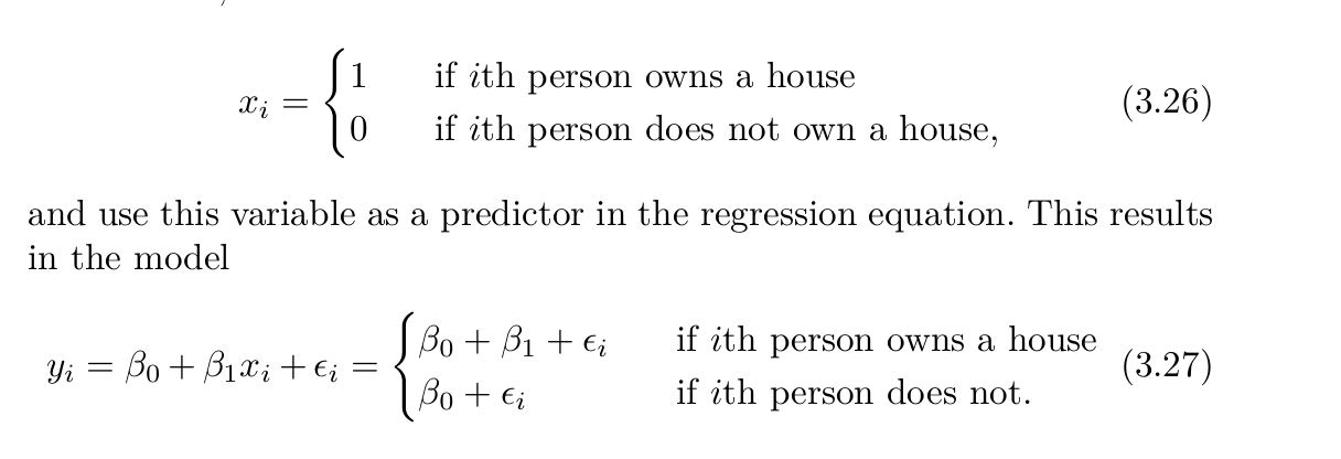
Now β0 can be interpreted as the average credit card balance among those who do not own, β0 + β1 as the average credit card balance among those who do own their house, and β1 as the average difference in credit card balance between owners and non-owners.
| Predictor | Coefficient | Std. Error | t-statistic | p-value |
| Intercept | 509.80 | 33.13 | 15.389 | <0.0001 |
| Own[Yes] | 19.73 | 46.05 | 0.429 | 0.6690 |
The average credit card debt for non-owners is estimated to be $509.80, whereas owners are estimated to carry $19.73 in additional debt for a total of $509.80 + $19.73 = $529.53. However, we notice that the p-value for the dummy variable is very high. This indicates that there is no statistical evidence of a difference in average credit card balance based on house ownership
Now β0 can be interpreted as the overall average credit card balance (ignoring the house ownership effect), and β1 is the amount by which house owners and non-owners have credit card balances that are above and below the average, respectively. In this example, the estimate for β0 is 519.665 dollar, halfway between the non-owner and owner averages of 509.80 dollar and 529.53. The estimate forβ1 is 9.865 dollar, which is half of 19.73 dollar, the average difference between owners and non-owners. It is important to note that the final pre dictions for the credit balances of owners and non-owners will be identical regardless of the coding scheme used. The only difference is in the way that the coefficients are interpreted
Qualitative Predictors with More than Two Levels
When a qualitative predictor has more than two levels, a single dummy variable cannot represent all possible values. In this situation, we can create additional dummy variables. For example, for the region variable we create two dummy variables. The first could be
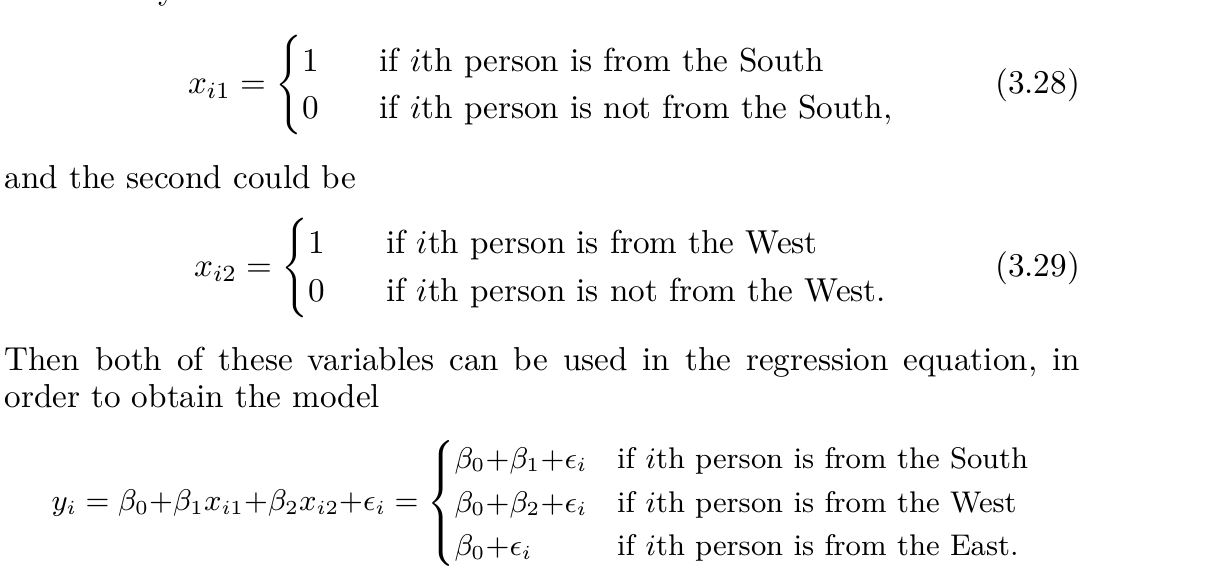
Now 0canbeinterpreted as the average credit card balance for individuals from the East, β1 can be interpreted as the difference in the average balance between people from the South versus the East, and β2 can be interpreted as the difference in the average balance between those from the West versus the East. There will always be one fewer dummy variable than the number of levels. The level with no dummy variable—East in this example—is known as the baseline
| Predictor | Coefficient | Std. Error | t-statistic | p-value |
| Intercept | 531.00 | 46.32 | 11.464 | <0.0001 |
| region[South] | -12.50 | 56.68 | -0.221 | 0.8260 |
| region[West] | -18.69 | 65.02 | -0.287 | 0.7740 |
1. Intercept (531.00): This is the baseline value when the region is not South or West (likely representing a reference category like "North" or "East"). The value 531.00 is the average prediction when the other variables are zero.
2.region[South] (-12.50): This value tells us that being in the South decreases the predicted value by 12.50 units compared to the reference category (e.g., North or East). However, the large p-value (0.8260) indicates that this effect is not statistically significant, meaning that we don't have enough evidence to say that the South region has a real impact on the outcome.
3. region[West] (-18.69): This suggests that being in the West decreases the predicted value by 18.69 units compared to the reference category. Similarly, the p-value (0.7740) is large, meaning this effect is also not statistically significant.
4. Summary: The intercept is significant, meaning the base value (for the reference region) is meaningful. However, the effects of the South and West regions on the outcome are not statistically significant, meaning there's no strong evidence that these regions have a real impact on the outcome in this model.
we see that the estimated balance for the baseline, East, is 531 dollar It is estimated that those in the South will have 18.69 less debt than those in the East, and that those in the West will have $12.50 less debt than those in the East. However, the p-values associated with the coefficient estimates for the two dummy variables are very large, suggesting no statistical evidence of a real difference in average credit card balance between South and East or between West and East.
Once again, the level selected as the baseline category is arbitrary, and the final predictions for each group will be the same regardless of this choice. However, the coefficients and their p-values do depend on the choice of dummy variable coding.
Using this dummy variable approach presents no difficulties when in corporation both quantitative and qualitative predictors. For example, to regress balance on both a quantitative variable such as income and a qualitative variable such as student, we must simply create a dummy variable for student and then fit a multiple regression model using income and the dummy variable as predictors for credit card balance.
----------------------------------------------------------------------------------
3.3.2 Extensions of the Linear Model.
----------------------------------------------------------------------------------
Two of the most important assumptions state that the relationship between the predictors and response are additive and linear. The additivity assumption means that the association between a predictor Xj and the response Y does not depend on the values of the other predictors. The linearity assumption states that the change in the response Y associated with a one-unit change in Xj is constant, regardless of the value of Xj. In later chapters of this book, we examine a number of sophisticated methods that relax these two assumptions. Here, we briefly examine some common classical approaches for extending the linear mode
Removing the Additive Assumption
In our previous analysis of the Advertising data, we concluded that both TVand radio seem to be associated with sales. The linear models that formed the basis for this conclusion assumed that the effect on sales of increasing one advertising medium is independent of the amount spent on the other media. For example, the linear model states that the average increase in sales associated with a one-unit increase in TV is always 1, regardless of the amount spent on radio.
However, this simple model may be incorrect. Suppose that spending money on radio advertising actually increases the effectiveness of TV advertising, so that the slope term for TV should increase as radio increases.
In this situation, given a fixed budget of $100,000, spending half on radio and half on TV may increase sales more than allocating the entire amount to either TV or to radio. In marketing, this is known as a synergy effect, and in statistics it is referred to as an interaction effect.
$$Y =B_{0} + B_{1} X_{1} + B_{2} X_{2} + \epsilon$$
According to this model, a one-unit increase in X1 is associated with an average increase in Y of β1 units. Notice that the presence of X2 doesn’t alter this statement—that is, regardless of the value of X2, a one unit increase in X1 is associated with a β1 -unit increase in Y . One way of extending this model is to include a third predictor, called an interaction term, which is constructed by computing the product of X1 and X2. This results in the model.
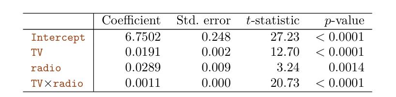
$$Y = B₀ + B₁ X₁ + B₂ X₂ + B₃ X₁ X₂ + ε$$
For example, suppose that we are interested in studying the productivity of a factory. We wish to predict the number of units produced on the basis of the number of production lines and the total number of workers. It seems likely that the effect of increasing the number of production lines will depend on the number of workers, since if no workers are available to operate the lines, then increasing the number of lines will not increase production. This suggests that it would be appropriate to include an inter action term between lines and workers in a linear model to predict units. Suppose that when we fit the model
Non-linear Relationships
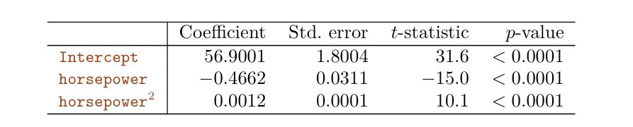
The approach that we have just described for extending the linear model to accommodate non-linear relationships is known as polynomial regression , since we have included polynomial functions of the predictors in the regression model
----------------------------------------------------------------------------------
3.3.3 Potential Problems.
----------------------------------------------------------------------------------
When we fit a linear regression model to a particular dataset, many problems may occur. Most common among these are the following:
1.Non-linearity of the response-predictor relationships.
2. Correlation of error terms.
3.Non-constant variance of error terms.
4.Outliers.
5.High-leveragepoints.
6. Collinearity.
1.Non-linearity of the response-predictor relationships.
The linear regression model assumes that there is a straight-line relationship between the predictors and the response. If the true relationship is far from linear, then virtually all of the conclusions that we draw from the fit are suspect. In addition, the prediction accuracy of the model can be significantly reduced.
Residual plots are a useful graphical tool for identifying non-linearity.
In the case of a multiple regression model, since there are multiple predictors, we instead plot the residuals versus the predicted (or fitted) values
If the residual plot indicates that there are non-linear associations in the data, then a simple approach is to use non-linear transformations of the predictors, such as logX, sqrt{X} , and X^2, in the regression model. In the later chapters of this book, we will discuss other more advanced non-linear approaches for addressing this issue.
6.Collinearity
Collinearity refers to the situation in which two or more predictor variables are closely related to one another.
The power of the hypothesis test—the probability of correctly detecting a non-zero coefficient—is reduced by collinearity.
A simple way to detect collinearity is to look at the correlation matrix of the predictors. An element of this matrix that is large in absolute value indicates a pair of highly correlated variables, and therefore a collinearity problem in the data.
Unfortunately, not all collinearity problems can be detected by inspection of the correlation matrix: it is possible for collinearity to exist between three or more variables even if no pair of variables has a particularly high correlation. We call this situation multicollinearity
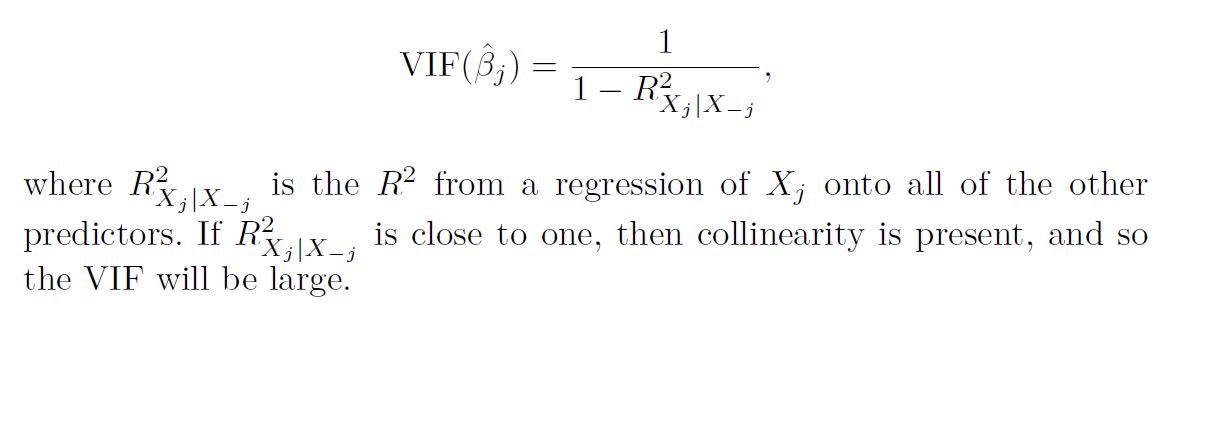
Instead of inspecting the correlation matrix, a better way to assess multi- collinearity collinearity is to compute the variance inflation factor (VIF)
The VIF is the ratio of the variance of β^j when fitting the full model divided by the variance of β^j if fit on its own.
The smallest possible value for VIF is 1, which indicates the complete absence of collinearity. Typically in practice there is a small amount of collinearity among the predictors. As a rule of thumb, a VIF value that exceeds 5 or 10 indicates a problematic amount of collinearity. The VIF for each variable can be computed using the formula
----------------------------------------------------------------------------------
3.4 The Marketing Plan.
----------------------------------------------------------------------------------
1. Is there a relationship between sales and advertising budget?
This question can be answered by fitting a multiple regression model of sales onto TV, radio, and newspaper
$$H_{0}: B_{TV} = B_{radio} = B_{newspaper} = 0$$
F-statistic can be used to determine whether or not we should reject this null hypothesis. In this case the p-value corresponding to the F-statistic is very low, indicating clear evidence of a relationship between advertising and sales.
2. How strong is the relationship?
We discussed two measures of model accuracy:
1. the RSE estimates the standard deviation of the response from the population regression line. For the Advertising data, the RSE is 1.69 units while the mean value for the response is 14.022, indicating a percentage error of roughly 12 %.
2. the R2 statistic records the percentage of variability in the response that is explained by the predictors. The predictors explain almost 90 % of the variance in sales.